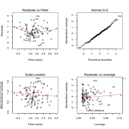
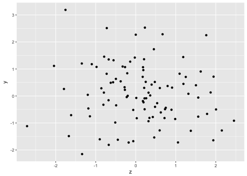
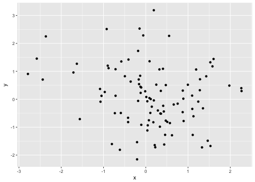
class: center, middle, inverse, title-slide # Miscellaneous Topics ## 😺 ### Tyson S. Barrett --- class: inverse # Outline -- ## Working with Dates -- ## Washing Data -- ## Loops, Loops, Loops, ... -- ## Joining Those Frames -- ## Modeling (assumptions, packages) --- class: inverse, middle, center # Working with Dates --- # Dates ```r library(lubridate) ``` .pull-left[ Extraction Functions: 1. `year()` 2. `month()` 3. `day()` 4. `hour()` 5. `minute()` 6. `second()` ] .pull-right[ Parsing (Working with Dates) Functions: 1. `ymd()` and its friends 2. `ymd_hms()` 3. `hms()` ] .footnote[[https://rpubs.com/davoodastaraky/lubridate](https://rpubs.com/davoodastaraky/lubridate)] --- # Extraction ```r right_now = now() right_now ``` ``` ## Warning in as.POSIXlt.POSIXct(x, tz): unknown timezone 'zone/tz/2017c.1.0/ ## zoneinfo/America/Denver' ``` ``` ## [1] "2017-12-12 06:57:18 GMT" ``` ```r str(right_now) ``` ``` ## POSIXct[1:1], format: "2017-12-12 06:57:18" ``` .pull-left[ ```r year(right_now) ``` ``` ## [1] 2017 ``` ```r month(right_now) ``` ``` ## [1] 12 ``` ```r day(right_now) ``` ``` ## [1] 12 ``` ] -- .pull-right[ ```r hour(right_now) ``` ``` ## [1] 6 ``` ```r minute(right_now) ``` ``` ## [1] 57 ``` ```r second(right_now) ``` ``` ## [1] 18.01454 ``` ] --- # Parsing (Working with) Dates Sometimes we need `R` to realize some variable is a date. This is where these functions are very valuable. ```r dates_but_not_dates = c("2017-12-13", "2017-12-14", "2017-12-15") ## what class is it? now_a_date = ymd(dates_but_not_dates) now_a_date ``` ``` ## [1] "2017-12-13" "2017-12-14" "2017-12-15" ``` ```r class(now_a_date) ``` ``` ## [1] "Date" ``` ```r str(now_a_date) ``` ``` ## Date[1:3], format: "2017-12-13" "2017-12-14" "2017-12-15" ``` --- # Parsing (Working with) Dates Lubridate is very flexible with formatting. ```r dates_but_not_dates = c("2017/12/3", "2017/12/14", "2017/12/15") ## what class is it? now_a_date = ymd(dates_but_not_dates) now_a_date ``` ``` ## [1] "2017-12-03" "2017-12-14" "2017-12-15" ``` ```r dates_but_not_dates = c("12031988", "12042010", "01032010") now_a_date = mdy(dates_but_not_dates) now_a_date ``` ``` ## [1] "1988-12-03" "2010-12-04" "2010-01-03" ``` ```r dates_but_not_dates = c(12032010, 12102010, 12202010) now_a_date = mdy(dates_but_not_dates) now_a_date ``` ``` ## [1] "2010-12-03" "2010-12-10" "2010-12-20" ``` --- # Time Distance Lubridate makes this very natural. ```r first = ymd("2010-12-03") last = today() last - first ``` ``` ## Time difference of 2566 days ``` ```r first = ymd_hms("2010-12-03 13:10:56 MST") last = now() last - first ``` ``` ## Time difference of 2565.741 days ``` --- class: inverse, middle, center # Washing Yo' Data --- # Washing Yo' Data Sometimes we need to change NAs to some other value, we need to remove NaNs, or replace place-holder values (999s) with NAs. .pull-left[ ```r df = data.frame( X = c(0, NA, 1, NA, 0, 1, 1, 0, 0, 0), Y = c(rnorm(9), NaN), Z = c(999, 1, 2, 1, 2, 1, 2, 1, 2, 1) ) df ``` ``` ## X Y Z ## 1 0 -0.9401621 999 ## 2 NA 0.1445659 1 ## 3 1 -0.3256783 2 ## 4 NA -0.7332431 1 ## 5 0 -0.9053486 2 ## 6 1 0.3307868 1 ## 7 1 -1.0477708 2 ## 8 0 -0.1253498 1 ## 9 0 -0.3207349 2 ## 10 0 NaN 1 ``` ] .pull-right[ ```r library(furniture) df %>% mutate(X = washer(X, is.na, value = 0), Y = washer(Y, is.nan, value = NA), Z = washer(Z, 999)) ``` ``` ## X Y Z ## 1 0 -0.9401621 NA ## 2 0 0.1445659 1 ## 3 1 -0.3256783 2 ## 4 0 -0.7332431 1 ## 5 0 -0.9053486 2 ## 6 1 0.3307868 1 ## 7 1 -1.0477708 2 ## 8 0 -0.1253498 1 ## 9 0 -0.3207349 2 ## 10 0 NA 1 ``` ] --- class: inverse, middle, center # Loops, Loops, Loops, ... --- # Looping ### Why do we use loops? 1. Want to repeat something over every column of a data frame 2. Need something done repeatedly -- ### What are our options? 1. `apply()` family of functions 2. `for` loops 3. manual --- # Loops ### `lapply()` - it repeats something over every column of the data frame - it can take built in functions and user functions -- .pull-left[ ```r df = data.frame( x = c(rnorm(99), NaN), y = c(rnorm(99), NaN) ) tail(df) ``` ``` ## x y ## 95 -0.20574815 -2.1522782 ## 96 -2.43808523 0.7050387 ## 97 -0.01381921 0.2844850 ## 98 -0.89939807 1.2026412 ## 99 0.04742223 -0.9346388 ## 100 NaN NaN ``` ] -- .pull-right[ ```r df2 = lapply(df, washer, is.nan) %>% data.frame tail(df2) ``` ``` ## x y ## 95 -0.20574815 -2.1522782 ## 96 -2.43808523 0.7050387 ## 97 -0.01381921 0.2844850 ## 98 -0.89939807 1.2026412 ## 99 0.04742223 -0.9346388 ## 100 NA NA ``` ] --- class: middle, center # Other Examples of Loops --- class: inverse, middle, center # Joining --- # Joining .pull-left[ ### Relational Tables .coral[Two or more connected data sets] ### Keys .coral[A variable, or group of variables, that define a single observation.] ] .pull-right[ ### Relations .coral[The way that one table's key is connected to another table] ### Functions .coral[The `*_join()` functions.] ] <br> <br> .foonote[See [R for Data Science](http://r4ds.had.co.nz/relational-data.html) book by Hadley Wickham, the chapter on relational data, for more information on this.] --- class: inverse, middle, center # Modeling --- # Modeling <div id="htmlwidget-1c5715fa81289de519fe" style="width:100%;height:auto;" class="datatables html-widget"></div> <script type="application/json" data-for="htmlwidget-1c5715fa81289de519fe">{"x":{"filter":"none","data":[["1","2","3","4","5","6","7","8","9","10"],["base","base","lavaan","lavaan","car","car","sandwich","lme4","lmerTest","geepack"],["lm","glm","cfa","sem","linearHypothesis","Anova","sandwich","lmer","lmer","geeglm"]],"container":"<table class=\"display\">\n <thead>\n <tr>\n <th> <\/th>\n <th>Package<\/th>\n <th>Function<\/th>\n <\/tr>\n <\/thead>\n<\/table>","options":{"dom":"t","order":[],"autoWidth":false,"orderClasses":false,"columnDefs":[{"orderable":false,"targets":0}]}},"evals":[],"jsHooks":[]}</script> --- # Modeling .large[ #### Checking Assumptions Each package is going to be slightly different but the good ones should have some information about checking assumptions. #### Basic Principles 1. Visualizations/tables are better than tests 2. Check data and model 3. Each method will have different assumptions and, thus, different techniques to assess them 4. Often, there is a lot of gray area here ] --- # Modeling #### Normality, Variance (Homoskedasticity), and Leverage ```r fit = lm(y ~ x + z, data = df2) par(mfrow = c(2,2)) plot(fit) ``` --- # Modeling #### Normality, Variance (Homoskedasticity), and Leverage <!-- --> --- # Modeling #### Normality, Variance (Homoskedasticity), and Leverage or via specialized functions (e.g., in SEM). ```r ## Not a great example library(lavaan) fit = sem("y ~ x + z", data = df2) modificationindices(fit) semTools::reliability(fit) semTools::measurementInvariance(fit) ``` --- # Modeling #### Linearity Check scatterplots. .pull-left[ ```r qplot(x = z, y = y, data = df2) ``` <!-- --> ] .pull-right[ ```r qplot(x = x, y = y, data = df2) ``` <!-- --> ] --- # Modeling Post Hoc Comparisons .large[Sometimes post hoc comparisons are important] -- ```r library(tidyverse) df3 = data_frame( x = sample(1:4, replace=TRUE, size = 100), grp = rbinom(100, 1, .5), y = x + grp + x * grp + rnorm(100) ) %>% mutate(x = factor(x), grp = factor(grp)) ``` ```r fit3 = aov(y ~ x * grp, data = df3) summary(fit3) ``` ``` ## Df Sum Sq Mean Sq F value Pr(>F) ## x 3 294.1 98.0 100.129 < 2e-16 *** ## grp 1 404.1 404.1 412.829 < 2e-16 *** ## x:grp 3 18.7 6.2 6.374 0.000567 *** ## Residuals 92 90.1 1.0 ## --- ## Signif. codes: 0 '***' 0.001 '**' 0.01 '*' 0.05 '.' 0.1 ' ' 1 ``` --- ```r TukeyHSD(fit3) ``` ``` ## Tukey multiple comparisons of means ## 95% family-wise confidence level ## ## Fit: aov(formula = y ~ x * grp, data = df3) ## ## $x ## diff lwr upr p adj ## 2-1 1.7543474 0.9435341 2.565161 0.0000010 ## 3-1 3.8960421 3.1743318 4.617752 0.0000000 ## 4-1 4.3099385 3.5723540 5.047523 0.0000000 ## 3-2 2.1416946 1.3873940 2.895995 0.0000000 ## 4-2 2.5555910 1.7860882 3.325094 0.0000000 ## 4-3 0.4138964 -0.2610717 1.088864 0.3811756 ## ## $grp ## diff lwr upr p adj ## 1-0 3.999622 3.605346 4.393897 0 ## ## $`x:grp` ## diff lwr upr p adj ## 2:0-1:0 0.754021152 -0.7055664 2.213609 0.7476855 ## 3:0-1:0 2.942591061 1.7140188 4.171163 0.0000000 ## 4:0-1:0 2.983789141 1.7764618 4.191116 0.0000000 ## 1:1-1:0 2.935917376 1.6218619 4.249973 0.0000000 ## 2:1-1:0 4.450841913 3.1979391 5.703745 0.0000000 ## 3:1-1:0 6.882964719 5.7392262 8.026703 0.0000000 ## 4:1-1:0 8.305103578 7.0977763 9.512431 0.0000000 ## 3:0-2:0 2.188569910 0.7498134 3.627326 0.0002212 ## 4:0-2:0 2.229767990 0.8091098 3.650426 0.0001228 ## 1:1-2:0 2.181896224 0.6694901 3.694302 0.0005604 ## 2:1-2:0 3.696820761 2.2372332 5.156408 0.0000000 ## 3:1-2:0 6.128943567 4.7619146 7.495973 0.0000000 ## 4:1-2:0 7.551082427 6.1304242 8.971741 0.0000000 ## 4:0-3:0 0.041198080 -1.1408610 1.223257 1.0000000 ## 1:1-3:0 -0.006673686 -1.2975518 1.284204 1.0000000 ## 2:1-3:0 1.508250852 0.2796786 2.736823 0.0059373 ## 3:1-3:0 3.940373658 2.8233409 5.057406 0.0000000 ## 4:1-3:0 5.362512517 4.1804534 6.544572 0.0000000 ## 1:1-4:0 -0.047871766 -1.3185471 1.222804 1.0000000 ## 2:1-4:0 1.467052771 0.2597255 2.674380 0.0067477 ## 3:1-4:0 3.899175577 2.8055524 4.992799 0.0000000 ## 4:1-4:0 5.321314437 4.1613519 6.481277 0.0000000 ## 2:1-1:1 1.514924537 0.2008690 2.828980 0.0125290 ## 3:1-1:1 3.947047343 2.7366283 5.157466 0.0000000 ## 4:1-1:1 5.369186203 4.0985109 6.639862 0.0000000 ## 3:1-2:1 2.432122806 1.2883843 3.575861 0.0000001 ## 4:1-2:1 3.854261666 2.6469344 5.061589 0.0000000 ## 4:1-3:1 1.422138860 0.3285157 2.515762 0.0027620 ``` --- # Modeling Post Hoc Comparisons ```r library(effects) comps = effects::Effect(c("x","grp"), fit3) cbind(comps$x, comps$fit, comps$lower, comps$upper) %>% set_names(c("x", "grp", "est", "lower", "upper")) %>% ggplot(aes(x=x, y=est, group=grp, color=grp, fill=grp)) + geom_line() + geom_point() + geom_errorbar(aes(ymin = lower, ymax = upper), width = .3) ``` --- # Modeling Post Hoc Comparisons <img src="06_Misc_files/figure-html/unnamed-chunk-27-1.png" style="display: block; margin: auto;" /> --- # Modeling .large[What modeling techniques do you use in your research?] <br> .large[Any specific examples you'd like to see?]