Chapter 1: The Basics
“Success is neither magical nor mysterious. Success is the natural consequence of consistently applying the basic fundamentals.” — Jim Rohn
R is an open source statistical software made by statisticians. This means it generally speaks the language of statistics. This is very helpful when it comes running analyses but can be confusing when starting to understand the code.
The best way to begin to learn R (in my opinion) is by jumping right into it and using it. To do so, as we learn new concepts, we will go through two main sections within each chapter:
- Introduction to the concept with examples of its use
- Application of the concept through projects provided at tysonbarrett.com
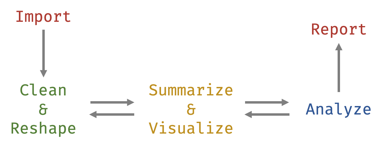
As we start working with data in R, we will go through several main themes, including importing and cleaning data, reshaping and otherwise wrangling3 data, assessing data via visualizations and tables, and running common statistical tests. We will follow the flow shown in the figure below.
As such, this chapter will provide the background and foundation to start using R. This background is important to get us to the first step in the data analysis lifecycle—that of importing data. Without this background, most of the other things we’d discuss would not make much sense. This background revolves around understanding data frames and functions—two general types of objects.
Objects
R is built on a few different types of virtual objects. An object, just like in the physical world, is something you can do things with. In the real world, we have objects that we use regularly. For example, we have chairs. Chairs are great for some things (sitting on, sleeping on, enjoying the beach) and horrible at others (playing basketball, flying, floating in the ocean). Similarly, in R each type of object is useful for certain things. The data types that we will discuss below are certain types of objects.

Chair
Because this is so analogous to the real world, it becomes quite natural to work with. You can have many objects in the computer’s memory, which allows flexbility in analyzing many different things simply within a single R session.4 The main object types that you’ll work with are presented in the following table (others exist that will come up here and there).
| Object | Description |
|---|---|
| Vector | A single column of data (‘a variable’) |
| Data Frame | Multiple vectors put together with observations as rows and variables as columns (much like a Spreadsheet that you have probably used before) |
| Function | Takes input and produces output—the workhorse of R |
| Operator | A special type of function (e.g. <-) |
Each of these objects will be introduced in this chapter, highlighting their definition and use. For your work, the first objects you work with will be data in various forms. Below, we explain the different data types and how they can combine into what is known as a data.frame.
Early Advice: Don’t get overwhelmed. It may feel like there is a lot to learn, but taking things one at a time will work surprisingly quickly. I’ve designed this book to discuss what you need to know from the beginning. Other topics that are not discussed are things you can learn later and do not need to be of your immediate concern.
Data Types
To begin understanding data in R, you must know about vectors. Vectors are, in essence, a single column of data—a variable. In R there are three main vector data types (variable types) that you’ll work with in research:
- numeric
- factor
- character
The first, numeric, is just that: numbers. In R, you can make a numeric variable with the code below:
x <- c(10.1, 2.1, 4.6, 2.3, 8.9, 4.5, 7.2, 7.9, 3.6, 2.0)The c() is a function5 that stands for “concatenate” which basically glues the values inside the paratheses together into one. We use <- to put it into x. So in this case, x (which we could have named anything) is saving those values so we can work with them6. If we ran this code, the x object would be in the working memory of R and will stay there unless we remove it or until the end of the R session (i.e., we close R).
A factor variable is a categorical variable (i.e., only a limited number of options exist). For example, race/ethnicity is a factor variable.
race <- c(1, 3, 2, 1, 1, 2, 1, 3, 4, 2)The code above actually produces a numeric vector (since it was only provided numbers). We can quickly tell R that it is indeed supposed to be a factor.
race <- factor(race,
               labels = c("white", "black", "hispanic", "asian"))
The factor() function tells R that the first thing—race—is actually a factor. The additional argument labels tells R what each of the values means. If we print out race we see that R has replaced the numeric values with the labels.
race## [1] white hispanic black white white black white
## [8] hispanic asian black
## Levels: white black hispanic asianFinally, and maybe less relevantly, there are character variables. These are words (known as strings). In research this is often where subjects give open responses to a question. These can be used somewhat like factors in a lot of situations.
ch <- c("I think this is great.",
        "I would suggest you learn R.",
        "You seem quite smart.")
When we combine multiple variables into one, we create a data.frame. A data frame is like a spreadsheet table, like the ones you have probably seen in Microsoft’s Excel and IBM’s SPSS. Here’s a simple example:
df <- data.frame(x, race)
df
## x race
## 1 10.1 white
## 2 2.1 hispanic
## 3 4.6 black
## 4 2.3 white
## 5 8.9 white
## 6 4.5 black
## 7 7.2 white
## 8 7.9 hispanic
## 9 3.6 asian
## 10 2.0 blackWe can do quite a bit with the data.frame that we called df7. Once again, we could have called this data frame anything (e.g., jimmy, susan, rock, scissors all would work), although I recommend short names. If we hadn’t already told R that race was a factor, we could do this once it is inside of df by:
df$race <- factor(df$race,
               labels = c("white", "black", "hispanic", "asian"))
In the above code, the $ reaches into df to grab a variable (or column). There are other ways of doing this as is almost always the case in R. For example, you may see individuals using:
df[["race"]] <- factor(df[["race"]] ,
                       labels = c("white", "black", "hispanic", "asian"))
df[["race"]] grabs the race variable just like df$race. Although there are many ways of doing this, we are going to focus on the modern and intuitive ways of doing this more often.
In my experience, the first element of uncomfort that researchers face is the fact that our data is essentially invisible to us. It is “housed” in df (not totally accurate but can be thought of this way for now) but it is hard to know exactly what is in df. First, we can use:
View(df)which prints out the data in spreadsheet-type form to see the data. We can also get nice summaries using the following functions.
names(df)## [1] "x" "race"str(df)## 'data.frame': 10 obs. of 2 variables:
## $ x : num 10.1 2.1 4.6 2.3 8.9 4.5 7.2 7.9 3.6 2
## $ race: Factor w/ 4 levels "white","black",..: 1 3 2 1 1 2 1 3 4 2summary(df)## x race
## Min. : 2.000 white :4
## 1st Qu.: 2.625 black :3
## Median : 4.550 hispanic:2
## Mean : 5.320 asian :1
## 3rd Qu.: 7.725
## Max. :10.100Functions
Earlier we mentioned that c() was a “function.” Functions are how we do things with our data. There are probably hundreds of thousands of functions at your reach. In fact, you can create your own! We’ll discuss that more in later chapters.
For now, know that each named function has a name (the function name of c() is “c”), arguments, and output of some sort. Arguments are the information that you provide the function between the parenthases (e.g. we gave c() a bunch of numbers; we gave factor() two arguments—the variable and the labels for the variable’s levels). Output from a function varies to a massive degree but, in general, the output is what you are using the function for (e.g., for c() we wanted to create a vector—a variable—of data where the arguments we gave it are glued together into a variable).
At any point, by typing:
?functionnamewe get information in the “Help” window. It provides information on how to use the function, including arguments, output, and examples.
Sometimes R by itself does not have a function that you need. We can download and use functions in packages8. We can think about packages as just that, a box of things. We will be using several functions from some very useful packages. To install them, we can use the install.packages() function,
install.packages("rio")This puts the package called rio on your computer for you. But without the next bit of code, the functions stay hidden in the package. To dump out all the functions in the package so we can use them, we use
library(rio)We now can use the functions from rio in this R session (i.e. from when you open R to when you close it).
After a quick note about operators, you will be shown several functions for both importing and saving data. Note that each have a name, arguments, and output of each.
Operators
A special type of function is called an operator. These take two inputs—a left hand side and a right hand side—and output some value. A very common operator is <-, known as the assignment operator. It takes what is on the right hand side and assigns it to the left hand side. We saw this earlier with vectors and data frames. Other operators exist, a few of which we will introduce in the following chapter. But again, an operator is just a special function.
Importing Data
Most of the time you’ll want to import data into R rather than manually entering it line by line, variable by variable.
We will rely on the rio package to do the majority of our data importing. In general, researchers in our fields use .csv, .txt, .sav, and .xlxs. For the most part, importing will be straightforward. Regardless of the file type, we will use rio::import(). Using the rio:: means we are reaching inside of the rio package and grabbing just one function, in this case import(). This is another way of grabbing a function instead of dumping out all the functions via library(rio).
The following code will read in the file your_data_file.csv. For now, it is easiest to work with data that you save in the same folder as your R script file or your RMarkdown file (both of which we will introduce in the Apply It section).
## Import your_data_file.csv
our_data <- rio::import("your_data_file.csv")
This will work for .csv, .txt, .sav, .xlsx, and many others files. In the example, we assigned our imported file to df using <-. This is necessary to let R remember the data for it to use for other stuff. The object our_data now contains the data saved in the CSV file called "your_data_file.csv". Note that at the end of the lines you see that I left a comment using #. I used two for stylistic purposes but only one is necessary. Anything after a # is not read by the computer; it’s just for us humans.
Heads up! It is important to know where your data file is located. In my experience, this is where students struggle the most at the very beginning. If the file is in the same folder as the RStudio project, we can use the
here::here()function to point to the project’s folder. More will be discussed about RStudio projects after the discussion on saving data.
If you have another type of data file to import that rio::import() doesn’t work well with, online helps found on sites like www.stackoverflow.com and www.r-bloggers.com often have the solution.
Saving Data
Occassionally you’ll want to save some data that you’ve worked with (usually this is not necessary). When necessary, you can use rio::export().
rio::export(df, file="file.csv") ## to create a CSV data fileR automatically saves missing data as NA since that is what it is in R. But often when we write a CSV file, we might want it as blank or some other value. If that’s the case, we can add another argument na = " " after the file argument.
Again, if you ever have questions about the specific arguments that a certain function has, you can simply run ?functionname. So, if you were curious about the different arguments in export simply run: ?export. In the pane with the files, plots, packages, etc. a document will show up to give you more informaton.
Apply it
This link contains a folder complete with an Rstudio project file, an RMarkdown file, and a few data files. Download it and unzip it to do the following steps.
Step 1
Open the Chapter1.Rproj file. This will open up RStudio for you within the “Chapter1” project.9
Step 2
Once RStudio has started, in the panel on the lower-right, there is a Files tab. Click on that to see the project folder. You should see the data files and the Chapter1.Rmd file. Click on the Chapter1.Rmd file to open it. It should open in the upper-left panel. The .Rmd stands for RMarkdown. It is a type of file where you can write code in code chunks (has ```{r} right above it) and write regular text elsewhere. This particular one that I’ve provided already has words and code put in it for you. Starting at the first code chunk, click on the first line and run the code. The code can be run using “Cmd +”Enter" or the Run button at the top of RStudio.
Step 3
Run the code to import the CSV file. At the end of that code chunk there is a link that is simply df. Run that line. It should print out some of the data in df. If you see the data printed out, you have done these steps correctly. Feel free to play around with this file and import the other data file types and run other code we’ve shown in this chapter.
Conclusions
R is designed to be flexible and do just about anything with data that you’ll need to do as a researcher. With this chapter under your belt, you can now read basic R code, import and save your data. The next chapter will introduce the “tidyverse” of methods that can help you join, reshape, summarize, group, and much more.
The hip term for working with data including selecting variables, filtering observations, creating new variables, etc.↩
An
Rsession is any time you openRdo work and then closeR. Unless you are saving your workspace (which, in general you shouldn’t do), it starts the slate clean–no objects are in memory and no packages are loaded. This is why we use scripts. Also, it makes your workflow extra transparent and replicable.↩Ris all about functions. Functions tellRwhat to do with the data. You’ll see many more examples throughout the book.↩This is a great feature of
R. It is called “object oriented” which basically meansRcreates objects to work with. I discuss this more in 1.2. Also, the fact that I saidx“saves” the information is not entirely true but is useful to think this way.↩I used this name since
dfis common in online helps and other resources.↩A package is an extension to
Rthat gives you more functions–abilities–to work with data. Anyone can write a package, although to get it on the Comprehensive R Archive Network (CRAN) it needs to be vetted to a large degree. In fact, after some practice, you could write a package to help you more easily do your work.↩A project just orients RStudio to that folder and helps you stay organized in your data analysis workflow.↩