Using Jamovi: Chi Square
30 Mar 2018This post is part of a series–demonstrating the use of Jamovi–mainly because some of my students asked for it. Notably, this is using version 0.8.6.0. Today’s topic is correlation and linear regression.
Note: This starts by assuming you know how to get data into Jamovi and start getting descriptive statistics.
Chi Square Goodness of Fit
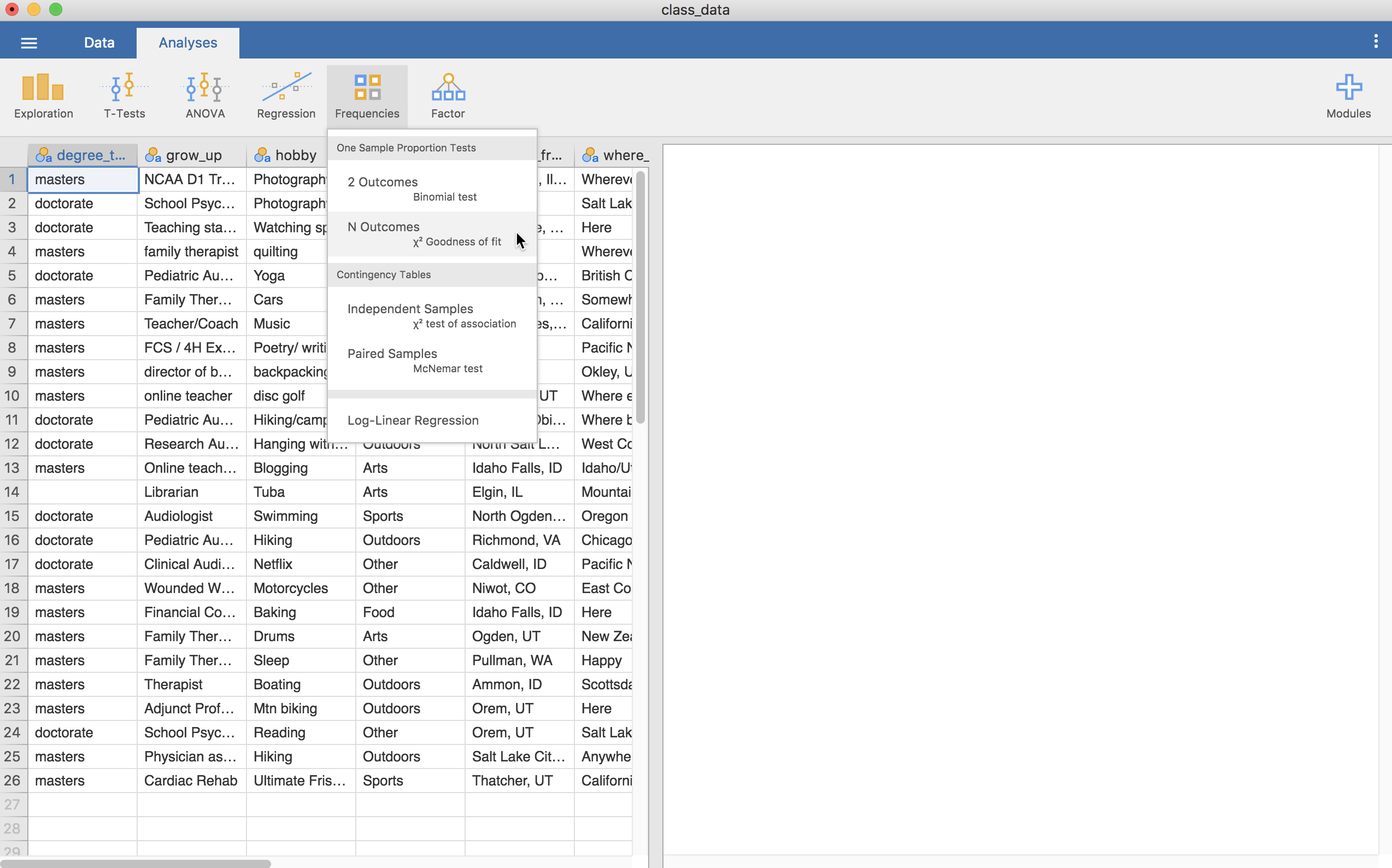
Running chi square goodness of fit tests in Jamovi requires only a few steps once the data is ready to go. To start, click on the Frequencies tab and then on N Outcomes as shown below.
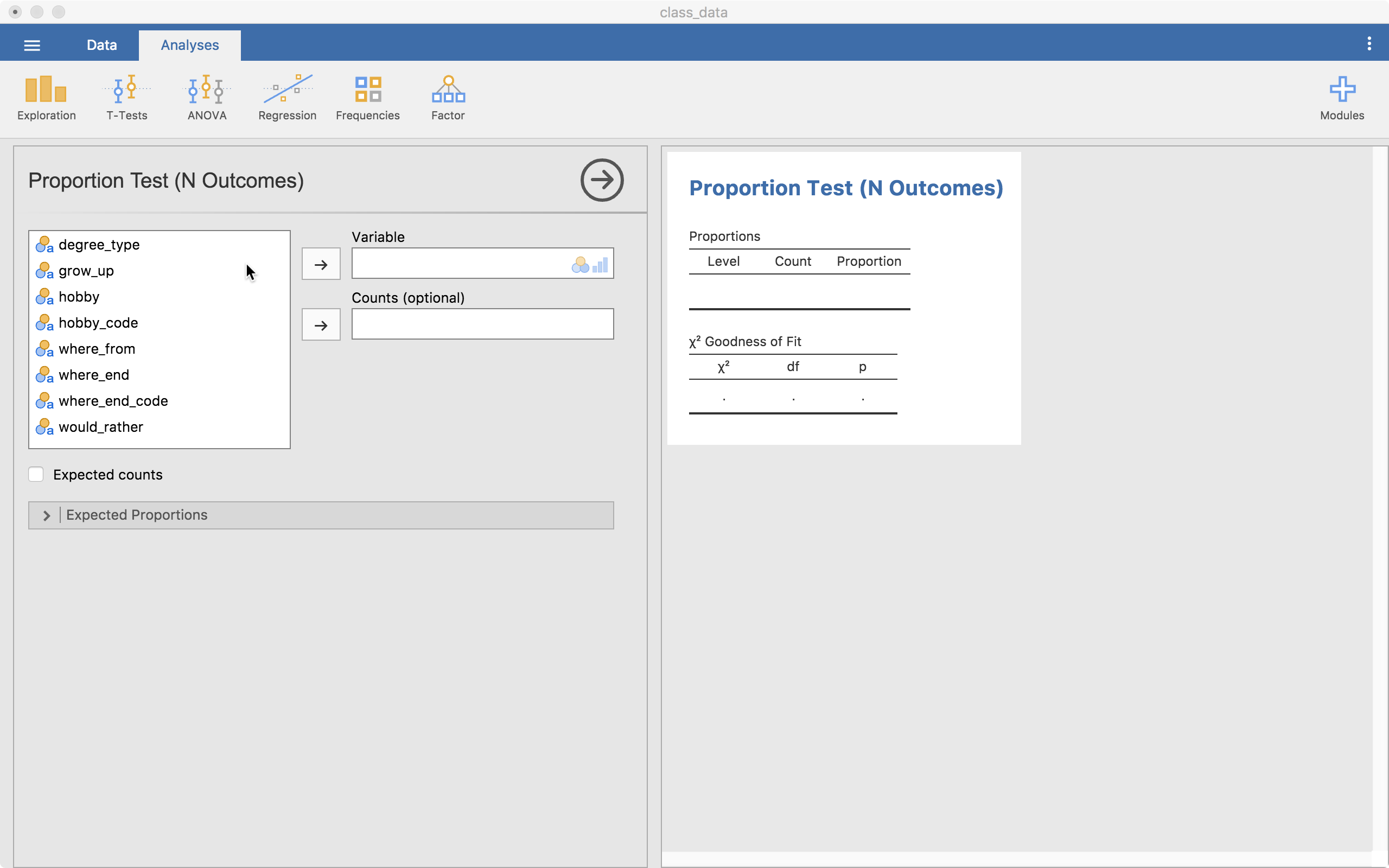
The following screen will then show up. This allows us to use two types of data—the raw data or summaries with counts. Herein, we will use the raw data. As such, all we need to do is add a nominal variable to the “Variable” slot.
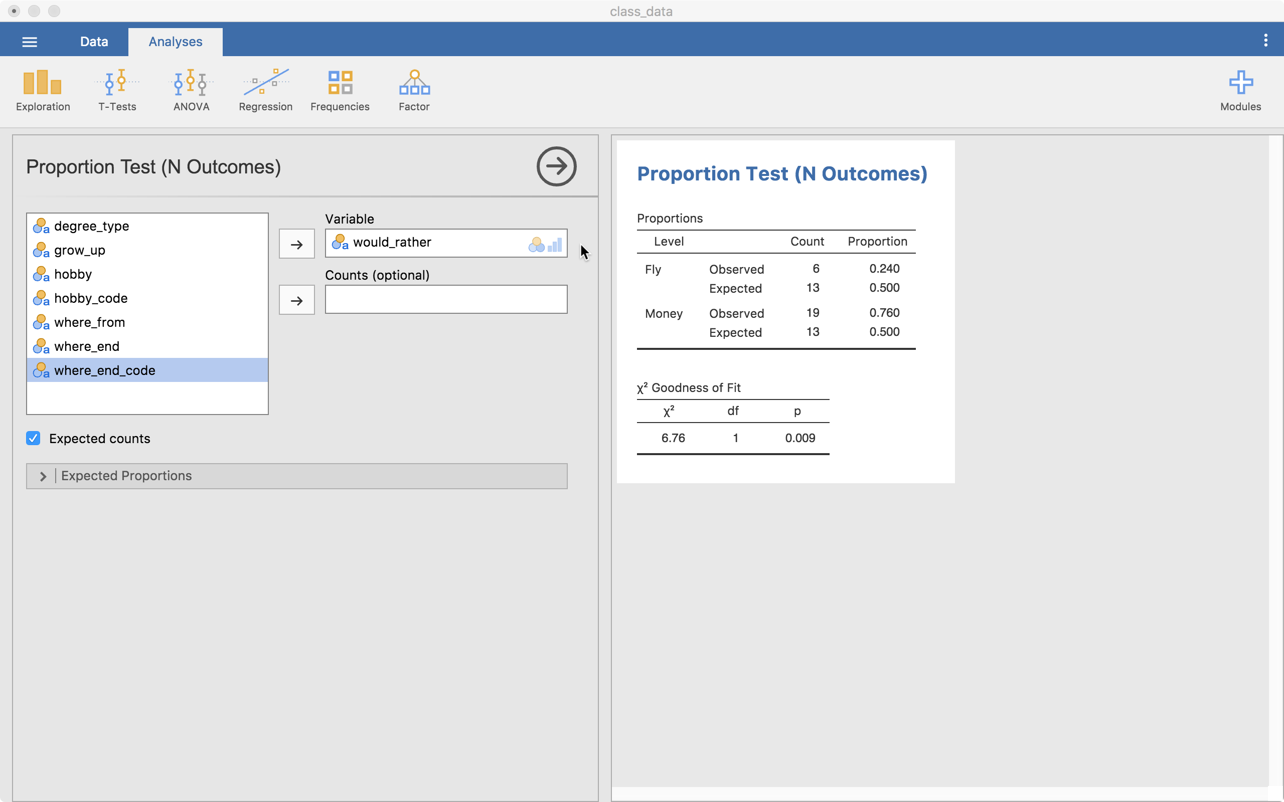
The goodness of fit test with a contingency table (cross-tabs table) both show up immediately for our would_rather variable (Would you rather be able to fly or have loads of money?). We also clicked the “Expected Counts” option, showing the observed and expected amounts. Here, the expected count for both options is 13. We observed 6 fly options and 19 money options. The table bottom table shows us our statistics and p-value (p = .009). This tells us that money showed up more often than we would expect by chance (i.e., there is a significant difference).
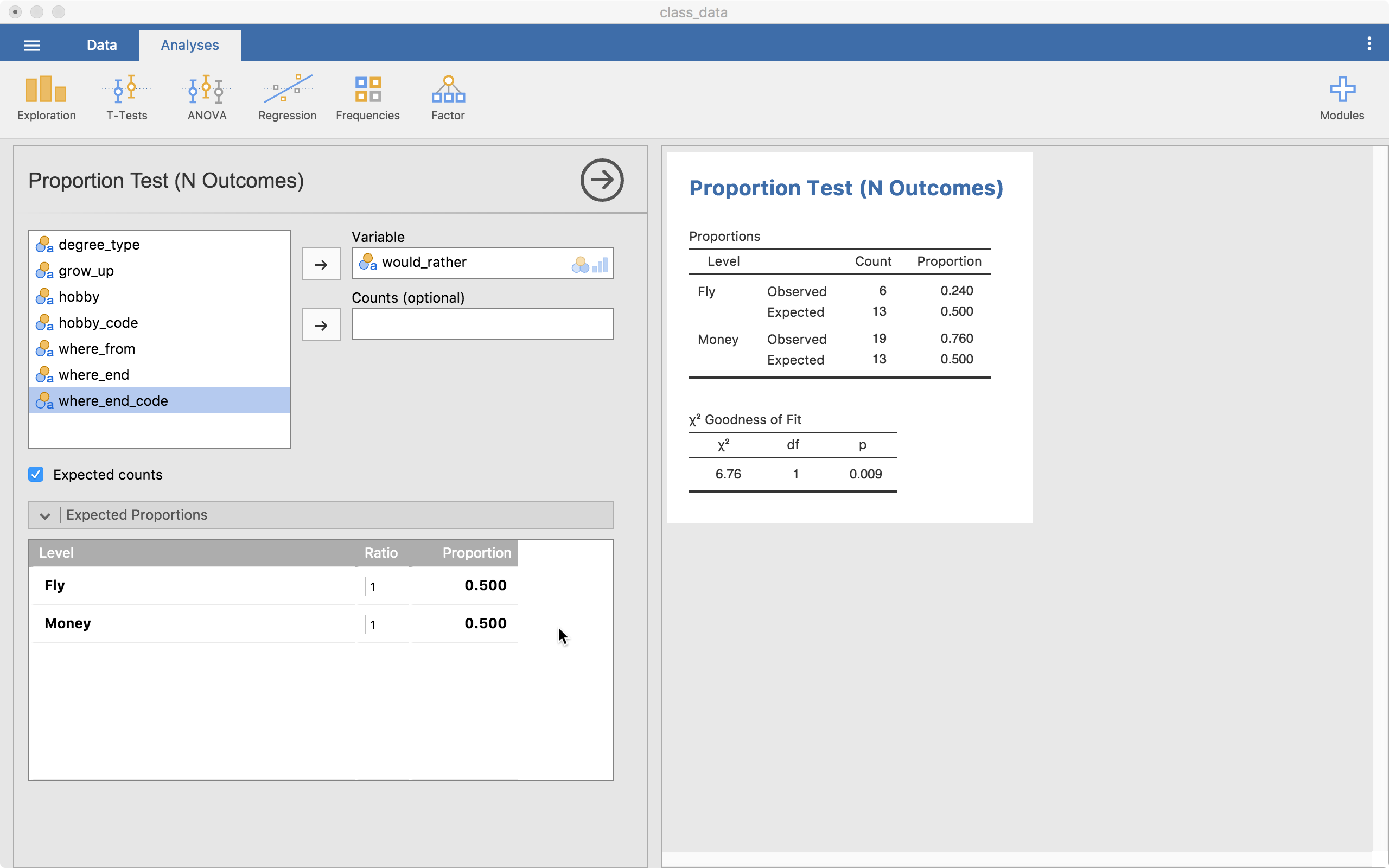
The menu below, “Expected Proportions” allows us to customize how many we expect from each category. The default is the same across all levels (a ratio of 1).
Chi Square Test of Independence
The test of independence is also in the Frequencies tab and then Independent Samples.
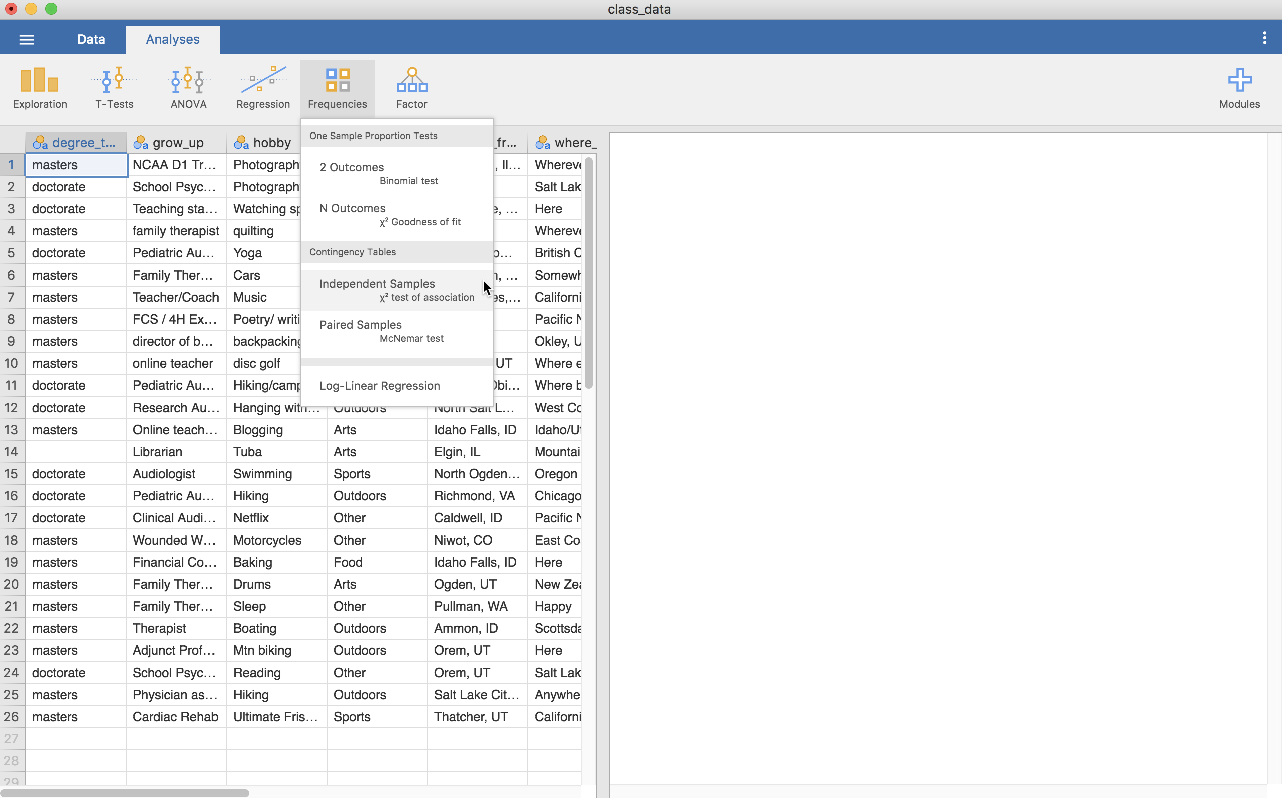
Clicking on this provides this screen (below) where we can put in two variables, one into “Rows” and another in “Columns” (“Counts” is used if we have summary data with counts for our variables; “Layers” allows us to do a chi square by group.)
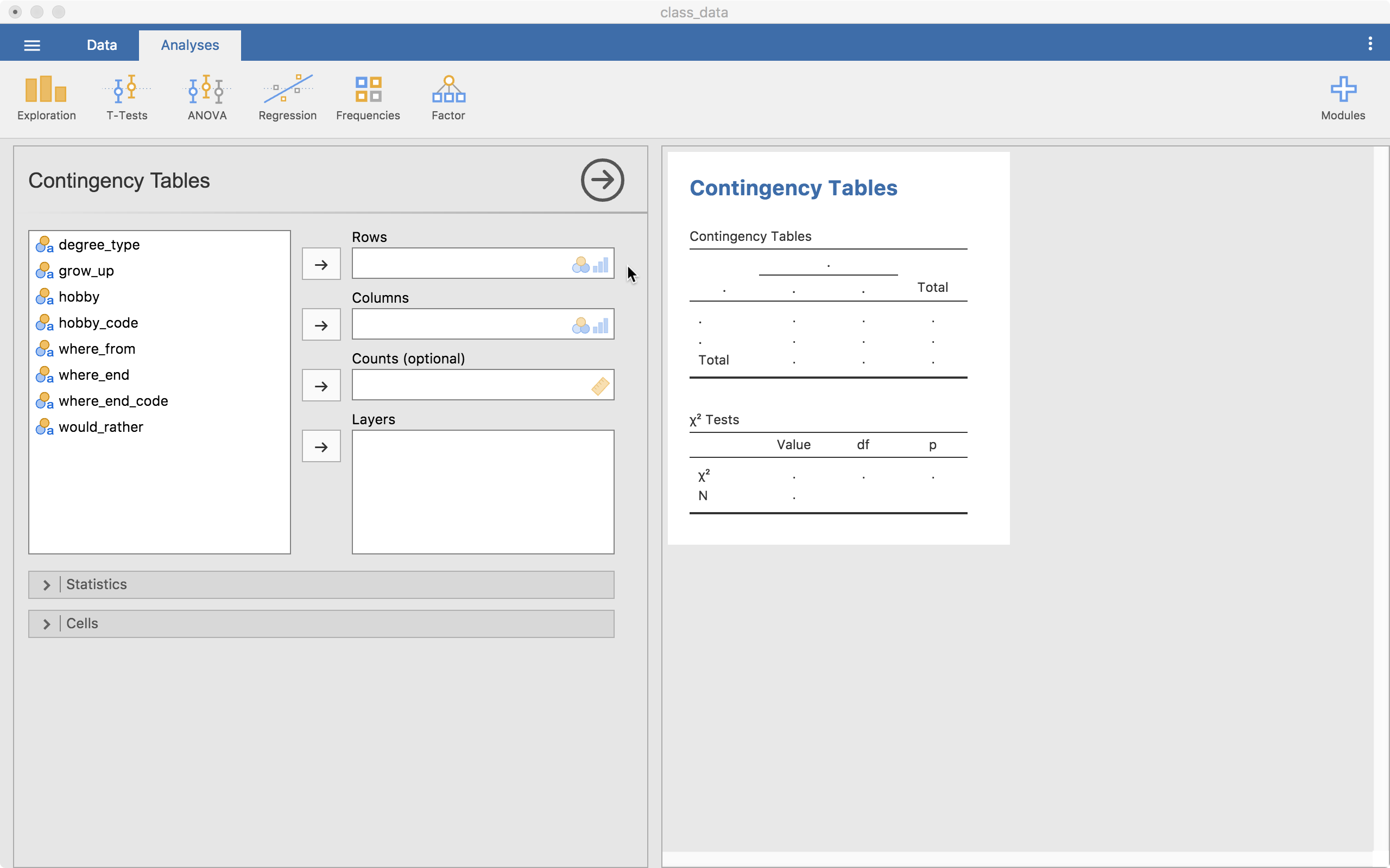
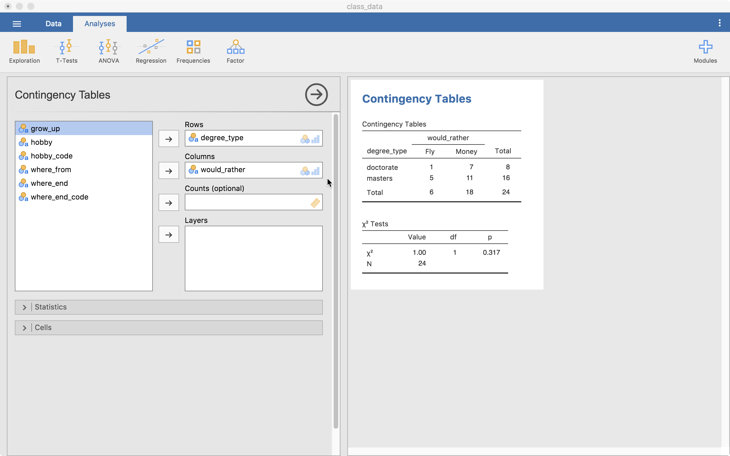
The test output is already up on the right. We have a contingency table (cross-tabs table) showing us the counts of each combination of the levels of the two variables. One problem is immediately clear, our expected counts for some of the cells may be small (we’ll see this output a little lower). If we ignore this problem, we can look at our test table showing us our chi-square statistic, df, and the p-value.
Statistics
The “Statistics” menu allows us to grab more information. For right now, we will just look at the “Nominal” options (all but the “Tests” options are essentially effect sizes). For a 2 by 2 table (like we have here), the Phi coefficient is useful so we will select that one.
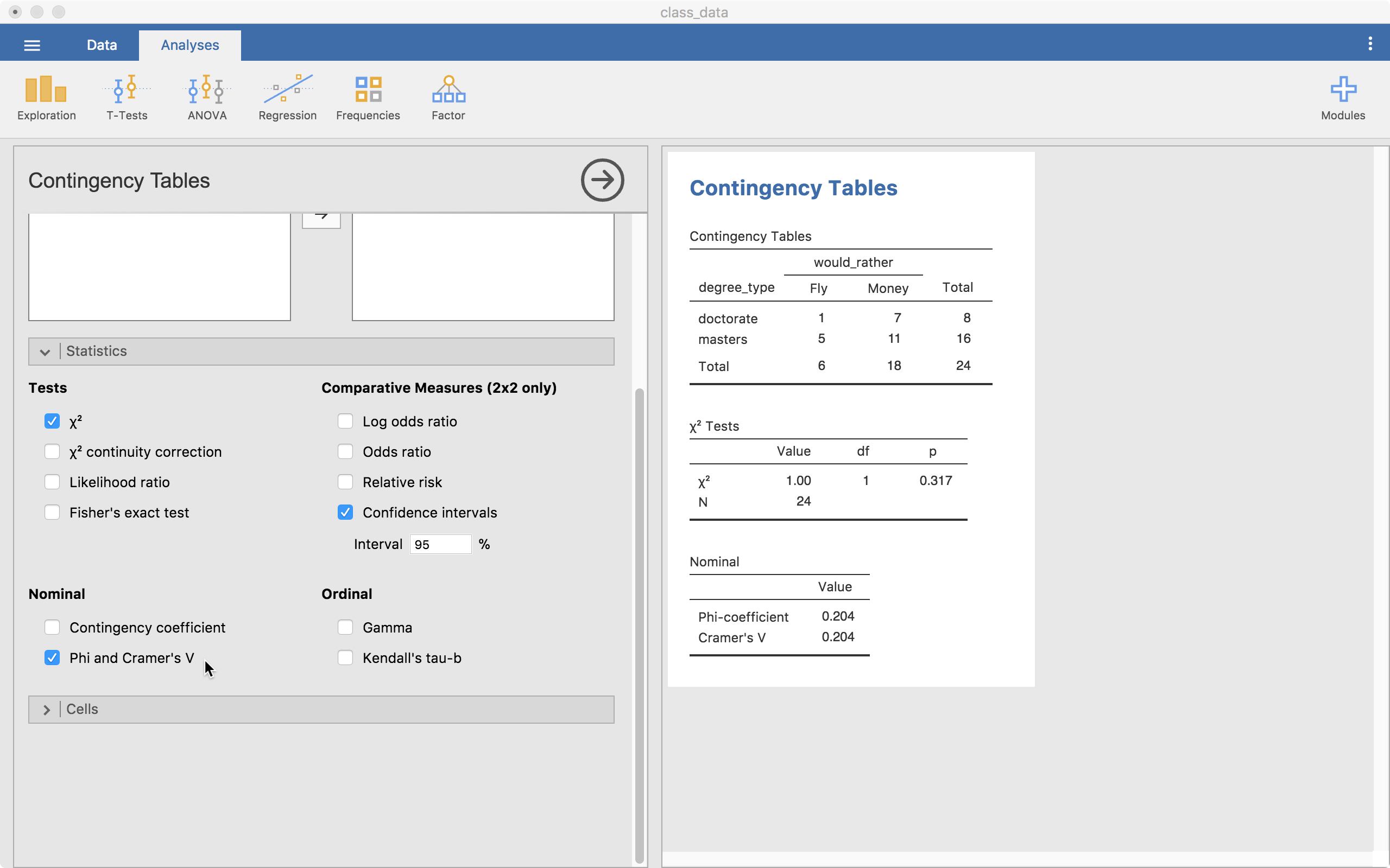
Our value is .204 which can be considered a small-to-moderate effect size.
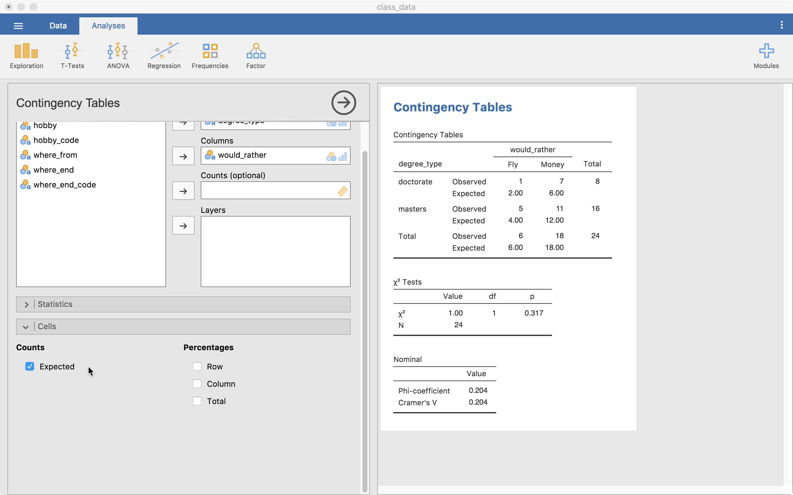
Cells
In the “Cells” menu, we can get more information in our contingency table. For our purposes, the “Expected” option is important (others can be). This is because we need to know if any of the expected frequencies is below 5. In this case, the Doctorate x Fly cell has an expected frequency of 2 so we know we have a problem. This tells us our p-value may not be valid.
Conclusions
Well, that’s it for now. Leave comments or questions below!