Chapter 2: Working with and Cleaning Your Data
“Organizing is what you do before you do something, so that when you do it, it is not all mixed up.” — A. A. Milne
In order to work with and clean your data in the most modern and straightforward way, we are going to be using the “tidyverse” group of methods. The tidyverse10 is a group of packages11 that provide a simple syntax that can do many basic (and complex) data manipulating. They form a sort of “grammar” of data manipulation that simplifies both the coding approach and the way researchers think about working with data.
The group of packages can be downloaded via:
install.packages("tidyverse")After downloading it, to use its functions, simply use:
library(tidyverse)## ── Attaching packages ─────────────────────────────────────────────────────────────────────── tidyverse 1.2.1.9000 ──## ✔ ggplot2 3.1.1 ✔ purrr 0.3.2
## ✔ tibble 2.1.1 ✔ dplyr 0.8.0.1
## ✔ tidyr 0.8.3 ✔ stringr 1.4.0
## ✔ readr 1.3.1 ✔ forcats 0.4.0## ── Conflicts ─────────────────────────────────────────────────────────────────────────────── tidyverse_conflicts() ──
## ✖ dplyr::filter() masks stats::filter()
## ✖ dplyr::lag() masks stats::lag()Note that when we loaded tidyverse it loaded several packages and told you of “conflicts”. These conflicts are where two or more functions across different packages have the same name. These functions with the same name will almost invariably differ in what they do. In this situation, the last loaded package is the one that R will use by default. For example, if we loaded two packages—awesome and amazing—and both had the function make_really_cool and we loaded awesome and then amazing as so:
library(awesome)
library(amazing)
R will automatically use the function from amazing. We can still access the awesome version of the function (because, again, even though the name is the same, they won’t necessarily do the same things for you). We can do this by:
awesome::make_really_cool(args)We showed this notation in Chapter 1. To review, the :: grabs the function from inside of the package and let’s you use just that function. That’s a bit of an aside, but know that you can always get at a function even if it is “masked” from your current session.
Tidy Methods
I’m introducing this to you for a couple reasons.
- It simplifies the code and makes the code more readable. It is often worthwhile to make sure the code is readable for, as the saying goes, there are always at least two collaborators on any project: you and future you.
- It is the cutting edge of all things
R. The most influential individuals in theRworld, including the makers and maintainers ofRStudio, use these methods and syntax.
The majority of what you’ll need to do with data as a researcher will be covered by these functions. The goal of these packages is to help tidy up your data. Tidy data is based on columns being variables and rows being observations. This depends largely on your data and research design but the definition is still the same—columns are variables and rows are observations. It is the form that data needs to be in to analyze it, whether that analysis is by graphing, modeling, or other means.
There are several methods that help create tidy data:
- Piping
- Selecting and Filtering
- Mutate and Transmute
- Grouping and Summarizing
- Reshaping
- Joining (merging)
Heads up! Understanding these tools requires an understanding of what ways data can be moved around. For example, reshaping can refer to moving data into a more wide-format or long-format, can refer to summarizing or aggregating, and can refer to joining or binding. All of these are necessary to work with data flexibly. Because of this, we suggest taking your time to fully understand what each function is doing with the data.
Much of these may be things you have done in other tools such as spreadsheets. The copy-and-paste approach is seriously error prone and is not reproducible. Taking your time to learn these methods will be well worth it.
Tidy (Long) Form
Before diving in, I want to provide some examples of tidy data (also known as “long form”) and how they are different from another form, often called “wide form.”
Only when the data is cross-sectional and each individual is a row does this distinction not matter much. Otherwise, if there are multiple measurement periods per individual (longitudinal design), or there are multiple individuals per cluster (clustered design), the distinction between wide and long is very important for modeling and visualization.
Wide Form
Wide form generally has one unit (i.e. individual) per row. This generally looks like:
##    ID   Var_Time1   Var_Time2
## 1   1 -1.82665774 0.009128897
## 2   2  1.68390857 0.933029763
## 3   3  1.75902687 0.249979359
## 4   4 -1.10090426 0.622896703
## 5   5  0.48963051 0.340643380
## 6   6 -0.87497855 0.379341163
## 7   7 -0.21235504 0.443984838
## 8   8  0.87680528 0.074131385
## 9   9  0.02772986 0.588852892
## 10 10 -1.91455731 0.486002357
Notice that each row has a unique ID, and some of the columns (all in this case) are variables at specific time points. This means that the variable is split up and is not a single column. This is a common way to collect and store data in our fields and so your data likely looks similar to this.
Long Form
In contrast, long format has the lowest nested unit as a single row. This means that a single ID can span multiple rows, usually with a unique time point for each row as so:
##   ID Time        Var
## 1  1    1 0.66379146
## 2  1    2 0.58118682
## 3  1    3 0.43395799
## 4  1    4 0.84304727
## 5  2    1 0.26147313
## 6  2    2 0.52240353
## 7  3    1 0.90175221
## 8  3    2 0.03428608
## 9  3    3 0.06609034
Notice that a single ID spans multiple columns and that each row has only one time point. Here, time is nested within individuals making it the lowest unit. Therefore, each row corresponds to a single time point. Generally, this is the format we want for most modeling techniques and most visualizations.
This is a very simple example of the differences between wide and long format. Although much more complex examples are probably available to you, we will start with this for now. Chapter 8 will delve into more complex data designs and how to reshape those. Toward the end of this chapter, we show reshaping with more simple data structures.
Data Used for Examples
To help illustrate each aspect of working with and cleaning your data, we are going to use real data from the National Health and Nutrition Examiniation Survey (NHANES). I’ve provided this data at https://tysonstanley.github.io/assets/Data/NHANES.zip. I’ve cleaned it up somewhat already.
Let’s quickly read that data in so we can use it throughout the remainder of this chapter.
library(rio)
dem_df <- import("NHANES_demographics_11.xpt")
med_df <- import("NHANES_MedHeath_11.xpt")
men_df <- import("NHANES_MentHealth_11.xpt")
act_df <- import("NHANES_PhysActivity_11.xpt")
Now we have four separate, but related, data sets in memory:
dem_dfcontaining demographic informationmed_dfcontaining medical health informationmen_dfcontaining mental health informationact_dfcontaining activity level information
Since all of them have all-cap variable names, we are going to quickly change this with a little trick:
names(dem_df) <- tolower(names(dem_df))
names(med_df) <- tolower(names(med_df))
names(men_df) <- tolower(names(men_df))
names(act_df) <- tolower(names(act_df))
This takes the names of the data frame (on the right hand side), changes them to lower case and then reassigns them to the names of the data frame.12
We will now go through each aspect of the tidy way of working with data using these four data sets.
Piping
Let’s introduce a few major themes in this tidyverse. First, the pipe operator – %>%. It helps simplify the code and makes things more readable. It takes what is on the left hand side and puts it in the right hand side’s function.
dem_df %>% head()So the above code takes the data frame dem_df and puts it into the head function. This does the same thing as head(df).
To illustrate its strength, consider the following example. We take dem_df, group it by gender, and then count.
dem_df %>%
  group_by(riagendr) %>%
  summarize(mean_age = mean(ridageyr, na.rm = TRUE))
## # A tibble: 2 x 2
## riagendr mean_age
## <dbl> <dbl>
## 1 1 31.1
## 2 2 31.7Without using the pipe, we would need to use something like:
summarize(group_by(dem_df, riagendr), mean_age = mean(ridageyr, na.rm = TRUE))## # A tibble: 2 x 2
## riagendr mean_age
## <dbl> <dbl>
## 1 1 31.1
## 2 2 31.7Although it is fewer lines, this is notably harder to understand. Instead of reading from left to right, top to bottom, we must read inside out, which is unnatural for English reading individuals.
Select Variables and Filter Observations
We often want to subset our data in some way before we do many of our analyses. We may want to do this for a number of reasons (e.g., easier cognitively to think about the data, the analyses depend on the subsetting). The code below show the two main ways to subset your data:
- selecting variables and
- filtering observations.
To select three variables (i.e. gender [“riagendr”], age [“ridageyr”], and ethnicity [“ridreth1”]) we:
selected_dem <- dem_df %>%
  select(riagendr, ridageyr, ridreth1)
Now, selected_dem has three variables and all the observations.
We can also filter (i.e. take out observations we don’t want):
filtered_dem <- dem_df %>%
  filter(riagendr == 1)
Since when riagendr == 1 the individual is male, filtered_dem only has male participants. We can add multiple filtering options as well:
filtered_dem <- dem_df %>%
  filter(riagendr == 1 & ridageyr > 16)
We now have only males that are older than 16 years old. We used & to say we want both conditions to be met. Alternatively, we could use:
filtered_dem <- dem_df %>%
  filter(riagendr == 1 | ridageyr > 16)
By using | we are saying we want males or individuals older than 16. In other words, if either are met, that observation will be kept.
Finally, we can do all of these in one step:
filtered_selected_dem <- dem_df %>%
  select(riagendr, ridageyr, ridreth1) %>%
  filter(riagendr == 1 & ridageyr > 16)
where we use two %>% operators to grab dem_df, select the three variables, and then filter the rows that we want.
Mutate Variables
Earlier we showed how to create a new variable or clean an existing one. We used the base R way for these. However, a great way to add and change variables is using mutate(). We grab df, and create a variable called citizen using the factored version of dmdcitzn and assign it back into df.
## Our Grouping Variable as a factor
dem_df <- dem_df %>%
  mutate(citizen = factor(dmdcitzn))
The benefit is in the readability of the code. We repeat things like the name of the data frame much less. I highly recommend working this way.
Grouping and Summarizing
A major aspect of analysis is comparing groups. Lucky for us, this is very simple in R. I call it the three step summary:
- Data
- Group by
- Summarize
## Three step summary:
dem_df %>%                           ## 1. Data
  group_by(citizen) %>%              ## 2. Group by
  summarize(N = n())                 ## 3. Summarize
## Warning: Factor `citizen` contains implicit NA, consider using
## `forcats::fct_explicit_na`## # A tibble: 4 x 2
## citizen N
## <fct> <int>
## 1 1 8685
## 2 2 1040
## 3 7 26
## 4 <NA> 5The output is very informative. The first column is the grouping variable and the second is the N (number of individuals) by group. We can quickly see that there are four levels, currently, to the citizen variable. After some reading of the documentation we see that 1 = Citizen and 2 = Not a Citizen. A value of 7 it turns out is a placeholder value for missing. And finally we have an NA category. It’s unlikely that we want those to be included in any analyses, unless we are particularly interested in the missingness on this variable. So let’s do some simple cleaning to get this where we want it. To do this, we will use the furniture package.
install.packages("furniture")dem_df <- dem_df %>%
mutate(citizen = washer(citizen, 7), ## Changes all 7's to NA's
citizen = washer(citizen, 2, value = 0)) ## Changes all 2's to 0'sNow, our citizen variable is cleaned, with 0 meaning not a citizen and 1 meaning citizen. Let’s rerun the code from above with the three step summary:
## Three step summary:
dem_df %>%                           ## 1. Data
  group_by(citizen) %>%              ## 2. Group by
  summarize(N = n())                 ## 3. Summarize
## Warning: Factor `citizen` contains implicit NA, consider using
## `forcats::fct_explicit_na`## # A tibble: 3 x 2
## citizen N
## <fct> <int>
## 1 0 1040
## 2 1 8685
## 3 <NA> 31Its clear that the majority of the subjects are citizens. We can also check multiple variables at the same time, just separating them with a comma in the summarize function.
## Three step summary:
dem_df %>%                           ## 1. Data
  group_by(citizen) %>%              ## 2. Group by
  summarize(N = n(),                 ## 3. Summarize
            Age = mean(ridageyr, na.rm=TRUE))
## Warning: Factor `citizen` contains implicit NA, consider using
## `forcats::fct_explicit_na`## # A tibble: 3 x 3
## citizen N Age
## <fct> <int> <dbl>
## 1 0 1040 37.3
## 2 1 8685 30.7
## 3 <NA> 31 40.4We used the n() function (which gives us counts) and the mean() function which, shockingly, gives us the mean. Note that if there are NA’s in the variable, the mean (and most other functions like it) will give the result NA. To have R ignore these, we tell the mean function to remove the NA’s when you compute this using na.rm=TRUE.
We can also use furniture::table1() to do the three-step summary. By default, table1() will give you the mean and SD of numeric variables and counts and percentages for factors.
## Three step summary:
dem_df %>%                           ## 1. Data
  group_by(citizen) %>%              ## 2. Group by
  table1(Age = ridageyr,             ## 3. Summarize
         Sex = factor(riagendr))
## Warning: Factor `citizen` contains implicit NA, consider using
## `forcats::fct_explicit_na`## Using dplyr::group_by() groups: citizen##
## ───────────────────────────────
## citizen
## 0 1
## n = 1040 n = 8685
## Age
## 37.3 (18.5) 30.7 (25.1)
## Sex
## 1 523 (50.3%) 4315 (49.7%)
## 2 517 (49.7%) 4370 (50.3%)
## ───────────────────────────────This pattern of grouping and summarizing is something that will follow us throughout the book. It’s a great way to get to know your data well and to make decisions on what to do next with your data.
Reshaping
Earlier we described the differences between wide and long (or tidy) form. Now that you have an idea of the differences, we are going to introduce how to change from one to the other. Several functions exist for just this purpose, including gather() from the tidyr package and reshape() in the default stats package. Since these can be limited in certain situations, we are going to teach two functions that can be used in nearly any reshaping situation. For now, though, we will keep in simple.
First, we will go from wide to long form using long() from the furniture package.13 We are using the ficticious data for the example of wide format from above.
#library(furniture)
df_wide <- data.frame("ID"=c(1:10),
                      "Var_Time1"=rnorm(10),
                      "Var_Time2"=runif(10))
df_long <- long(df_wide,
                c("Var_Time1", "Var_Time2"),
                v.names = "Var")
## id = IDdf_long## ID time Var
## 1.1 1 1 -0.333951741
## 2.1 2 1 -1.426568720
## 3.1 3 1 -1.636822429
## 4.1 4 1 -0.103076854
## 5.1 5 1 -0.863310448
## 6.1 6 1 -1.174153676
## 7.1 7 1 0.799312003
## 8.1 8 1 -0.819714178
## 9.1 9 1 0.733398183
## 10.1 10 1 -0.002236534
## 1.2 1 2 0.818095696
## 2.2 2 2 0.072766873
## 3.2 3 2 0.198322854
## 4.2 4 2 0.602794213
## 5.2 5 2 0.365043242
## 6.2 6 2 0.174424975
## 7.2 7 2 0.251205900
## 8.2 8 2 0.488671686
## 9.2 9 2 0.234222258
## 10.2 10 2 0.936877253We provided the data (df_wide), the time varying variables (c("Var_Time1", "Var_Time2")), and told it what we should name the value variable (v.names = "Var"). Note that the function guessed, based on its name, that the variable ID was the identifying variable.
This function automatically assumes each observation is a time point, thus the time variable. We can easily change that by adding the argument timevar and giving it a name (e.g., timevar = "cluster").
And now we will go from long to wide using wide() from the same package.
df_long <- data.frame("ID"=c(1,1,1,1,2,2,3,3,3),
                      "Time"=c(1,2,3,4,1,2,1,2,3),
                      "Var"=runif(9))
df_wide <- wide(df_long,
                v.names = c("Var"),
                timevar = "Time")
## id = IDdf_wide## ID Var.1 Var.2 Var.3 Var.4
## 1 1 0.8994227 0.7214949 0.4274312 0.9213086
## 5 2 0.4962018 0.9713351 NA NA
## 7 3 0.8376052 0.3542951 0.8857001 NAHere, we provided the data df_long and the variable name (Var) that had the values and (Time) that contained the time labels (in this case, just numbers). With a little bit of code we can move data around without any copy-pasting that is so error-prone. Again, note that the function guessed, based on its name, that the variable ID was the identifying variable.
Joining (merging)
The final topic in the chapter is joining data sets. This is common in many situations including large surveys (e.g., a demographics set, physical activity set, family characteristics set), health records (financial data, doctors notes, diagnosis data), and longitudinal studies (data from wave I, data from wave II).
We currently have 4 data sets that have mostly the same people in them but with different variables. One tells us about the demographics; another gives us information on mental health. We may have questions that ask whether a demographic characteristics is related to a mental health factor. This means we need to merge, or join, our data sets.14
When we merge a data set, we combine them based on some ID variable(s). Here, this is simple since each individual is given a unique identifier in the variable seqn. Within the dplyr package (part of the tidyverse) there are four main joining functions: inner_join, left_join, right_join and full_join. Each join combines the data in slightly different ways.
The figure below shows each type of join in Venn Diagram form. Each are discussed below.
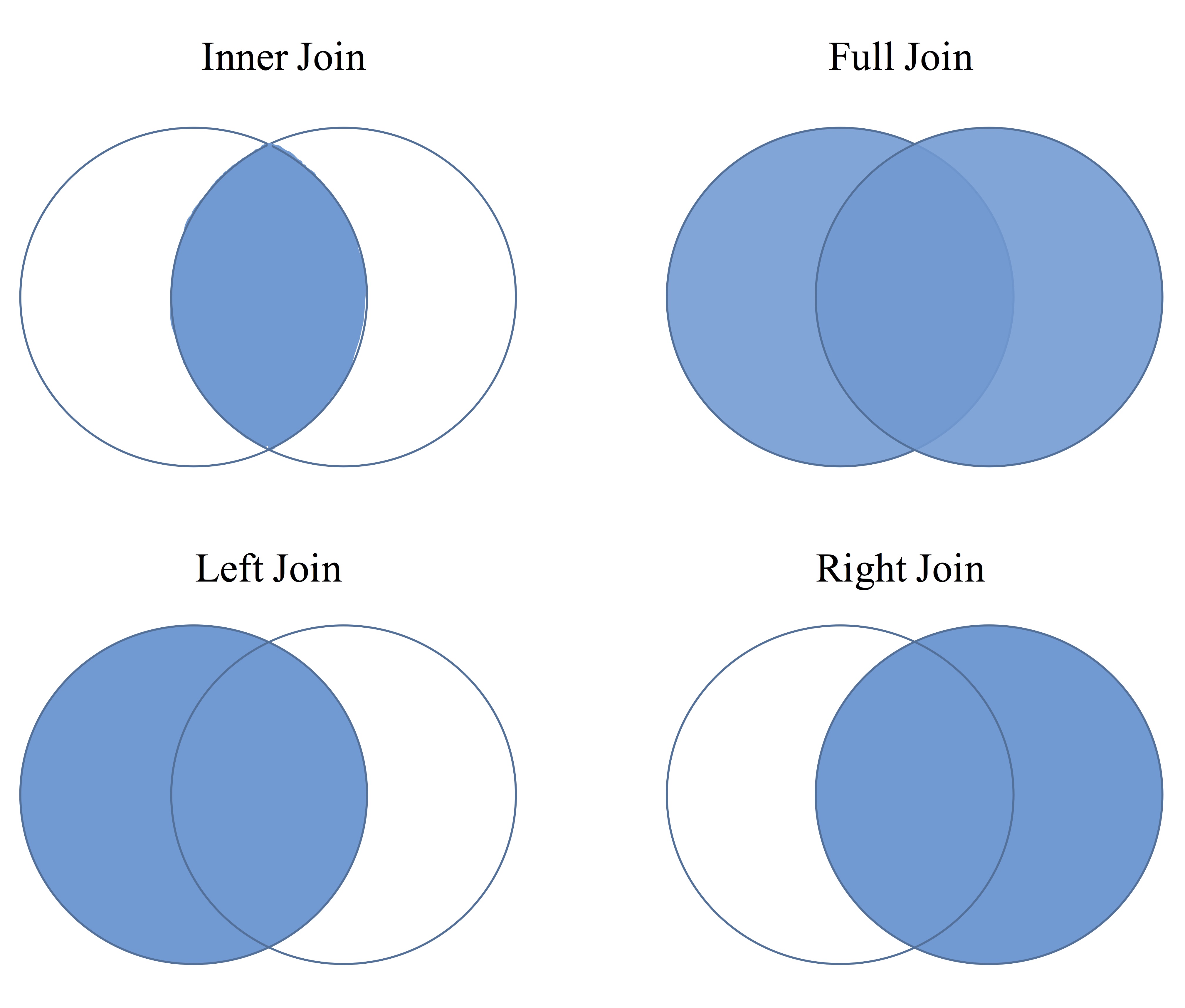
Joining
Inner Join
Here, only those individuals that are in both data sets that you are combining will remain. So if person “A” is in data set 1 and not in data set 2 then he/she will not be included.
inner_join(df1, df2, by="IDvariable")Left or Right Join
This is similar to inner join but now if the individual is in data set 1 then left_join will keep them even if they aren’t in data set 2. right_join means if they are in data set 2 then they will be kept whether or not they are in data set 1.
left_join(df1, df2, by="IDvariable")   ## keeps all in df1
right_join(df1, df2, by="IDvariable")  ## keeps all in df2
Full Join
This one simply keeps all individuals that are in either data set 1 or data set 2.
full_join(df1, df2, by="IDvariable")Each of the left, right and full joins will have missing values placed in the variables where that individual wasn’t found. For example, if person “A” was not in df2, then in a full join they would have missing values in the df1 variables.
For our NHANES example, we will use full_join to get all the data sets together. Note that in the code below we do all the joining in the same overall step.
df <- dem_df %>%
  full_join(med_df, by="seqn") %>%
  full_join(men_df, by="seqn") %>%
  full_join(act_df, by="seqn")
So now df is the the joined data set of all four. We started with dem_df joined it with med_df by seqn then joined that joined data set with men_df by seqn, and so on.
For many analyses in later chapters, we will use this new df object that is the combination of all the data sets that we had before. Whenever this is the case, this data will be explicitly referenced. Note, that in addition to what was shown in this chapter, a few other cleaning tasks were done on the data. This final version of df can be found at tysonstanley.github.io/R.
Wrap it up
Let’s put all the pieces together that we’ve learned in the chapter together on this new df data frame we just created. Below, we using piping, selecting, filtering, grouping, and summarizing.
First, let’s create an overall depression variable that is the sum of all the depression items (we could do IRT or some other way of combining them but that is not the point here). Below, we do three things:
- We clean up each depression item using
furniture::washer()since both “7” and “9” are placeholders for missing values. We take override the original variable with the cleaned one. - Next, we sum all the items into a new variable called
dep. - Finally, we create a dichotomized variable called
dep2using nestedifelse()functions. Theifelse()statements read: if condition holds (depis greater than or equal to10), then1, else if condition holds (depis less than10), then0, elseNA. The basic build of the function is:ifelse(condition, value if true, value if false).
In the end, we are creating a new data frame called df2 with the new and improved df with the items cleaned and depression summed and dichotomized.
df2 <- df %>%
  mutate(dpq010 = washer(dpq010, 7,9),
         dpq020 = washer(dpq020, 7,9),
         dpq030 = washer(dpq030, 7,9),
         dpq040 = washer(dpq040, 7,9),
         dpq050 = washer(dpq050, 7,9),
         dpq060 = washer(dpq060, 7,9),
         dpq070 = washer(dpq070, 7,9),
         dpq080 = washer(dpq080, 7,9),
         dpq090 = washer(dpq090, 7,9),
         dpq100 = washer(dpq100, 7,9)) %>%
  mutate(dep = dpq010 + dpq020 + dpq030 + dpq040 + dpq050 +
               dpq060 + dpq070 + dpq080 + dpq090) %>%
  mutate(dep2 = factor(ifelse(dep >= 10, 1,
                       ifelse(dep < 10, 0, NA))))
After these adjustments, let’s select, filter, group by, and summarize.
df2 %>%
  select(ridageyr, riagendr, mcq010, dep) %>%
  filter(ridageyr > 10 & ridageyr < 40) %>%
  group_by(riagendr) %>%
  summarize(asthma = mean(mcq010, na.rm=TRUE),
            depr   = mean(dep, na.rm=TRUE))
## # A tibble: 2 x 3
## riagendr asthma depr
## <dbl> <dbl> <dbl>
## 1 1 1.82 2.61
## 2 2 1.82 3.58We can see that males (riagendr = 1) have nearly identical asthma levels but lower depression levels than their female counterparts.
General Cleaning of the Data Set
A package known as janitor provides some nice functions that add to the ideas presented in this chapter. Specifically, two functions are of note:
clean_names()– cleans up the names of the data frame to make them easier to type and make sure it works well withR.remove_empty()– removes either empty columns or empty rows (columns or rows that have only missing values).
These can be used in tandem, like so:
df3 <- df2 %>%
  janitor::clean_names() %>%
  janitor::remove_empty("cols") %>%
  janitor::remove_empty("rows")
Ultimately, I hope you see the benefit to using these methods. With these methods, you can clean, reshape, and summarize your data. Because these are foundational, we will apply these methods throughout the book.
Apply It
This link contains a folder complete with an Rstudio project file, an RMarkdown file, and a few data files. Download it and unzip it to do the following steps.
Step 1
Open the Chapter2.Rproj file. This will open up RStudio for you.
Step 2
Once RStudio has started, in the panel on the lower-right, there is a Files tab. Click on that to see the project folder. You should see the data files and the Chapter2.Rmd file. Click on the Chapter2.Rmd file to open it. In this file, import the data, create a new variable, select three varaibles, and summarize a variable using the three step summary.
Once that code is in the file, click the knit button. This will create an HTML file with the code and output knitted together into one nice document. This can be read into any browser and can be used to show your work in a clean document.
Hadley Wickham (2016). tidyverse: Easily Install and Load ‘Tidyverse’ Packages. R package version 1.0.0. https://CRAN.R-project.org/package=tidyverse↩
Remember, a package is an extension to
Rthat gives you more functions that you can easily load intoR.↩Note that these are not particularly helpful names, but they are the names provided in the original data source. If you have questions about the data, visit http://wwwn.cdc.gov/Nchs/Nhanes/Search/Nhanes11_12.aspx.↩
Although the furniture package isn’t in the
tidyverse, it is a valuable package to use with the othertidyversepackages.↩Note that this is different than adding new rows but not new variables. Merging requires that we have at least some overlap of individuals in both data sets.↩