Chapter 8: Advanced Data Manipulation
“Every new thing creates two new questions and two new opportunities.” — Jeff Bezos
There’s so much more we can do with data in R than what we’ve presented. Two main topics we need to clarify here are:
- How do you reshape your data from wide to long form or vice versa in more complex data structures?
- How do can we automate tasks that we need done many times?
We will introduce both ideas to you in this chapter. To discuss the first, show the use of long() and wide() from the furniture package. For the second, we need to talk about loops. Looping, for our purposes, refers to the ability to repeat something across many variables or data sets. There’s many ways of doing this but some are better than others. For looping, we’ll talk about:
- vectorized functions,
forloops, and- the
applyfamily of functions.
Reshaping Your Data
We introduced you to wide form and long form of your data in Chapter 2. In reality, data can take on nearly infinite forms but for most data in health, behavioral, and social science, these two forms are sufficient to know.
In some situations, your data may have multiple variables with multiple time points (known as time-variant variables) and other variables that are not (known as time-invariant variables) as shown:
##    ID Var_Time1 Var_Time2 Var2_Time1 Var2_Time2     Var3
## 1   1   1.10900   0.96277    -0.9305    0.22067  0.05009
## 2   2  -0.27493   0.66534    -1.2622    0.66120  0.21316
## 3   3   0.51459   0.29909    -0.1249    0.78298 -0.80491
## 4   4  -1.12694   0.17760     1.1640   -1.74347  1.57872
## 5   5  -0.02065   0.87825    -0.7661    0.21988  0.84180
## 6   6  -0.13046   0.62382     0.1969    1.38130 -0.79274
## 7   7  -0.62082   0.08845    -0.8459    0.96443 -1.57274
## 8   8   0.92253   0.83129    -0.3986    0.27513  0.84952
## 9   9  -0.48041   0.97502    -0.5953   -0.03353  2.68741
## 10 10   0.55952   0.31066     1.5120   -1.57442  0.33950
Notice that this data frame is in wide format (each ID is one row and there are multiple times or measurements per person for two of the variables). To change this to wide format, we’ll use long(). The first argument is the data.frame, followed by two variable names (names that we go into the new long form), and then the numbers of the columns that are the measures (e.g., Var_Time1 and Var_Time2).
long_form <- furniture::long(d1,
                             c("Var_Time1", "Var_Time2"),
                             c("Var2_Time1", "Var2_Time2"),
                             v.names = c("Var", "Var2"))
## id = IDlong_form## ID Var3 time Var Var2
## 1.1 1 0.05009 1 1.10900 -0.93047
## 2.1 2 0.21316 1 -0.27493 -1.26217
## 3.1 3 -0.80491 1 0.51459 -0.12487
## 4.1 4 1.57872 1 -1.12694 1.16404
## 5.1 5 0.84180 1 -0.02065 -0.76613
## 6.1 6 -0.79274 1 -0.13046 0.19692
## 7.1 7 -1.57274 1 -0.62082 -0.84587
## 8.1 8 0.84952 1 0.92253 -0.39865
## 9.1 9 2.68741 1 -0.48041 -0.59531
## 10.1 10 0.33950 1 0.55952 1.51199
## 1.2 1 0.05009 2 0.96277 0.22067
## 2.2 2 0.21316 2 0.66534 0.66120
## 3.2 3 -0.80491 2 0.29909 0.78298
## 4.2 4 1.57872 2 0.17760 -1.74347
## 5.2 5 0.84180 2 0.87825 0.21988
## 6.2 6 -0.79274 2 0.62382 1.38130
## 7.2 7 -1.57274 2 0.08845 0.96443
## 8.2 8 0.84952 2 0.83129 0.27513
## 9.2 9 2.68741 2 0.97502 -0.03353
## 10.2 10 0.33950 2 0.31066 -1.57442As you can see, it took the variable names and put that in our first variable that we called “measures”. The actual values of the variables are now in the variable we called “values”. Finally, notice that each ID now has two rows (one for each measure).
To go in the opposite direction (long to wide) we can use the wide() function. All we do is provide the long formed data frame, variables that are time-varying (Var1 and Var2) and the variable showing the time points (time).
wide_form <- furniture::wide(long_form,
                             v.names = c("Var", "Var2"),
                             timevar = "time")
## id = IDwide_form## ID Var3 Var.1 Var2.1 Var.2 Var2.2
## 1.1 1 0.05009 1.10900 -0.9305 0.96277 0.22067
## 2.1 2 0.21316 -0.27493 -1.2622 0.66534 0.66120
## 3.1 3 -0.80491 0.51459 -0.1249 0.29909 0.78298
## 4.1 4 1.57872 -1.12694 1.1640 0.17760 -1.74347
## 5.1 5 0.84180 -0.02065 -0.7661 0.87825 0.21988
## 6.1 6 -0.79274 -0.13046 0.1969 0.62382 1.38130
## 7.1 7 -1.57274 -0.62082 -0.8459 0.08845 0.96443
## 8.1 8 0.84952 0.92253 -0.3986 0.83129 0.27513
## 9.1 9 2.68741 -0.48041 -0.5953 0.97502 -0.03353
## 10.1 10 0.33950 0.55952 1.5120 0.31066 -1.57442And we are back to the wide form.
These steps can be followed for situations where there are many measures per person, many people per cluster, etc. In most cases, this is the way multilevel data analysis occurs (as we discussed in Chapter 6) and is a nice way to get our data ready for plotting.
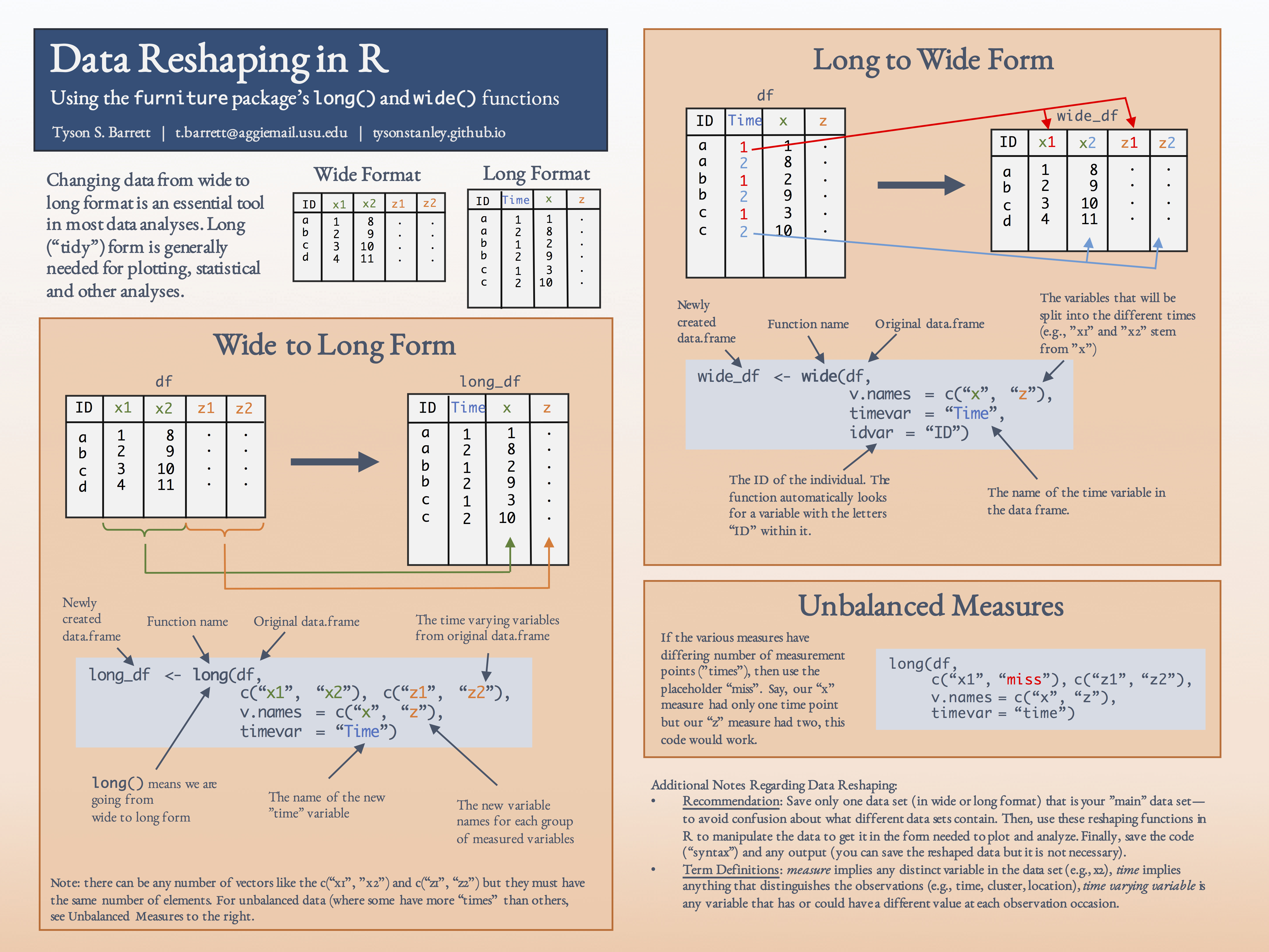
The following figure shows the features of both long() and wide().
Repeating Actions (Looping)
To fully go into looping, understanding how to write your own functions is needed.
Your Own Functions
Let’s create a function that estimates the mean (although it is completely unnecessary since there is already a perfectly good mean() function).
mean2 <- function(x){
  n <- length(x)
  m <- (1/n) * sum(x)
  return(m)
}
We create a function using the function() function.23 Within the function() we put an x. This is the argument that the function will ask for. Here, it is a numeric vector that we want to take the mean of. We then provide the meat of the function between the {}. Here, we did a simple mean calculation using the length(x) which gives us the number of observations, and sum() which sums the numbers in x.
Let’s give it a try:
v1 <- c(1,3,2,4,2,1,2,1,1,1)   ## vector to try
mean2(v1)                      ## our function
## [1] 1.8mean(v1) ## the base R function## [1] 1.8Looks good! These functions that you create can do whatever you need them to (within the bounds that R can do). I recommend by starting outside of a function that then put it into a function. For example, we would start with:
n <- length(v1)
m <- (1/n) * sum(v1)
m
## [1] 1.8and once things look good, we would put it into a function like we had before with mean2. It is an easy way to develop a good function and test it while developing it.
By creating your own function, you can simplify your workflow and can use them in loops, the apply functions and the purrr package.
For practice, we will write one more function. Let’s make a function that takes a vector and gives us the N, the mean, and the standard deviation.
important_statistics <- function(x, na.rm=FALSE){
  N  <- length(x)
  M  <- mean(x, na.rm=na.rm)
  SD <- sd(x, na.rm=na.rm)

  final <- c(N, M, SD)
  return(final)
}
One of the first things you should note is that we included a second argument in the function seen as na.rm=FALSE (you can have as many arguments as you want within reason). This argument has a default that we provide as FALSE as it is in most functions that use the na.rm argument. We take what is provided in the na.rm and give that to both the mean() and sd() functions. Finally, you should notice that we took several pieces of information and combined them into the final object and returned that.
Let’s try it out with the vector we created earlier.
important_statistics(v1)## [1] 10.000 1.800 1.033Looks good but we may want to change a few aesthetics. In the following code, we adjust it so we have each one labeled.
important_statistics2 <- function(x, na.rm=FALSE){
  N  <- length(x)
  M  <- mean(x, na.rm=na.rm)
  SD <- sd(x, na.rm=na.rm)

  final <- data.frame(N, "Mean"=M, "SD"=SD)
  return(final)
}
important_statistics2(v1)
## N Mean SD
## 1 10 1.8 1.033We will come back to this function and use it in some loops and see what else we can do with it.
Vectorized
By construction, R is the fastest when we use the vectorized form of doing things. For example, when we want to add two variables together, we can use the + operator. Like most functions in R, it is vectorized and so it is fast. Below we create a new vector using the rnorm() function that produces normally distributed random variables. First argument in the function is the length of the vector, followed by the mean and SD.
v2 <- rnorm(10, mean=5, sd=2)
add1 <- v1 + v2
round(add1, 3)## [1] 7.202 8.790 9.402 7.539 7.671 8.207 8.863 2.933 4.768 5.642We will compare the speed of this to other ways of adding two variables together and see it is the simplest and quickest.
For Loops
For loops have a bad reputation in the R world. This is because, in general, they are slow. It is among the slowest of ways to iterate (i.e., repeat) functions. We start here to show you, in essence, what the apply family of functions are doing, often, in a faster way.
At times, it is easiest to develop a for loop and then take it and use it within the apply or purrr functions. It can help you think through the pieces that need to be done in order to get your desired result.
For demonstration, we are using the for loop to add two variables together. The code between the ()’s tells R information about how many loops it should do. Here, we are looping through 1:10 since there are ten observations in each vector. We could also specify this as 1:length(v1). When using for loops, we need to keep in mind that we need to initialize a variable in order to use it within the loop. That’s precisely what we do with the add2, making it a numberic vector with 10 observations.
add2 <- vector("numeric", 10) ## Initialize
for (i in 1:10){
add2[i] <- v1[i] + v2[i]
}
round(add2, 3)## [1] 7.202 8.790 9.402 7.539 7.671 8.207 8.863 2.933 4.768 5.642Same results! But, we’ll see later that the speed is much than the vectorized function.
The apply family
The apply family of functions that we’ll introduce are:
apply()lapply()sapply()tapply()
Each essentially do a loop over the data you provide using a function (either one you created or another). The different versions are extremely similar with some minor differences. For apply() you tell it if you want to iterative over the columns or rows; lapply() assumes you want to iterate over the columns and outputs a list (hence the l); sapply() is similar to lapply() but outputs vectors and data frames. tapply() has the most differences because it can iterative over columns by a grouping variable. We’ll show apply(), lapply() and tapply() below.
For example, we can add two variables together here. We provide it the data.frame that has the variables we want to add together.
df <- data.frame(v1, v2)
add3 <- apply(df, 1, sum)
round(add3, 3)## [1] 7.202 8.790 9.402 7.539 7.671 8.207 8.863 2.933 4.768 5.642The function apply() has three main arguments: a) the data.frame or list of data, b) 1 meaning to apply the function for each row or 2 to the columns, and c) the function to use.
We can also use one of our own functions such as important_statistics2() within the apply family.
lapply(df, important_statistics2)## $v1
##    N Mean    SD
## 1 10  1.8 1.033
##
## $v2
## N Mean SD
## 1 10 5.302 1.792This gives us a list of two elements, one for each variable, with the statistics that our function provides. With a little adjustment, we can make this into a data.frame using the do.call() function with "rbind".
do.call("rbind", lapply(df, important_statistics2))## N Mean SD
## v1 10 1.800 1.033
## v2 10 5.302 1.792tapply() allows us to get information by a grouping factor. We are going to add a factor variable to the data frame we are using df and then get the mean of the variables by group.
group1 <- factor(sample(c(0,1), 10, replace=TRUE))
tapply(df$v1, group1, mean)
## 0 1
## 2.2 1.4We now have the means by each group. This, however, is probably replaced by the 3 step summary that we learned earlier in dplyr using group_by() and summarize().
These functions are useful in many situations, especially where there are no vectorized functions. You can always get an idea of whether to use a for loop or an apply function by giving it a try on a small subset of data to see if one is better and/or faster.
Speed Comparison
We can test to see how fast functions are with the microbenchmark package. Since it wants functions, we will create a function that uses the for looop.
forloop <- function(var1, var2){
  add2 <- vector("numeric", length(var1))
  for (i in 1:10){
    add2[i] <- var1[i] + var2[i]
  }
  return(add2)
}
Below, we can see that the vectorized version is nearly 50 times faster than the for loop and 300 times faster than the apply. Although the for loop was faster here, sometimes it can be slower than the apply functions–it just depends on the situation. But, the vectorized functions will almost always be much faster than anything else. It’s important to note that the + is also a function that can be used as we do below, highlighting the fact that anything that does something to an object in R is a function.
library(microbenchmark)
microbenchmark(forloop(v1, v2),
               apply(df, 1, sum),
               `+`(v1, v2))
## Unit: nanoseconds
## expr min lq mean median uq max neval cld
## forloop(v1, v2) 1701 2162.5 49725.3 2468 2772 4728220 100 a
## apply(df, 1, sum) 67769 69918.0 74822.2 71348 73118 191510 100 a
## v1 + v2 164 270.5 393.7 364 448 3074 100 aOf course, as it says the units are in nanoseconds. Whether a function takes 200 or 200,000 nanoseconds probably won’t change your life. However, if the function is being used repeatedly or on on large data sets, this can make a difference.
Using “Anonymous Functions” in Apply
Last thing to know here is that you don’t need to create a named function everytime you want to use apply. We can use what is called “Anonymous” functions. Below, we use one to get at the N and mean of the data.
lapply(df, function(x) rbind(length(x), mean(x, na.rm=TRUE)))## $v1
## [,1]
## [1,] 10.0
## [2,] 1.8
##
## $v2
## [,1]
## [1,] 10.000
## [2,] 5.302So we don’t name the function but we design it like we would a named function, just minus the return(). We take x (which is a column of df) and do length() and mean() and bind them by rows. The first argument in the anonymous function will be the column or variable of the data you provide.
Here’s another example:
lapply(df, function(y) y * 2 / sd(y))## $v1
## [1] 1.936 5.809 3.873 7.746 3.873 1.936 3.873 1.936 1.936 1.936
##
## $v2
## [1] 6.921 6.461 8.260 3.949 6.328 8.043 7.658 2.157 4.205 5.180We take y (again, the column of df), times it by two and divide by the standard deviation of y. Note that this is gibberish and is not some special formula, but again, we can see how flexible it is.
The last two examples also show something important regarding the output:
- The output will be at the level of the anonymous function. The first had two numbers per variable because the function produced two summary statistics for each variable. The second we multiplied
yby 2 (so it is still at the individual observation level) and then divide by the SD. This keeps it at the observation level so we get ten values for every variable. - We can name the argument anything we want (as long as it is one word). We used
xin the first andyin the second but as long as it is the same within the function, it doesn’t matter what you use.
Finally, we may not want our variables to be in the list format. We may want to control more tightly what is outputted from the looping. For that, we can thank the purrr package (part of the tidyverse; note the three r’s in purrr). This package provides many valuable functions that you can explore. Of particular mention here, though, are some of the map*() functions that work just like lapply().
map()– outputs a listmap_df()– outputs a data framemap_if()– outputs a list but only makes any changes to the variables that meet a condition (e.g.,is.numeric()).
purrr::map(df, function(y) y * 2 / sd(y))## $v1
## [1] 1.936 5.809 3.873 7.746 3.873 1.936 3.873 1.936 1.936 1.936
##
## $v2
## [1] 6.921 6.461 8.260 3.949 6.328 8.043 7.658 2.157 4.205 5.180purrr::map_df(df, function(y) y * 2 / sd(y))## # A tibble: 10 x 2
## v1 v2
## <dbl> <dbl>
## 1 1.94 6.92
## 2 5.81 6.46
## 3 3.87 8.26
## 4 7.75 3.95
## 5 3.87 6.33
## 6 1.94 8.04
## 7 3.87 7.66
## 8 1.94 2.16
## 9 1.94 4.20
## 10 1.94 5.18purrr::map_if(df, is.numeric, function(y) y * 2 / sd(y))## $v1
## [1] 1.936 5.809 3.873 7.746 3.873 1.936 3.873 1.936 1.936 1.936
##
## $v2
## [1] 6.921 6.461 8.260 3.949 6.328 8.043 7.658 2.157 4.205 5.180Apply It
This link contains a folder complete with an Rstudio project file, an RMarkdown file, and a few data files. Download it and unzip it to do the following steps.
Step 1
Open the Chapter8.Rproj file. This will open up RStudio for you.
Step 2
Once RStudio has started, in the panel on the lower-right, there is a Files tab. Click on that to see the project folder. You should see the data files and the Chapter8.Rmd file. Click on the Chapter8.Rmd file to open it. In this file, import the data, reshape it to long form, create your own function to do something for you, and apply the function in a loop over some of the variables of the data set.
Once that code is in the file, click the knit button. This will create an HTML file with the code and output knitted together into one nice document. This can be read into any browser and can be used to show your work in a clean document.
Conclusions
These are useful tools to use in your own data manipulation beyond that what we discussed with dplyr. It takes time to get used to making your own functions so be patient with yourself as you learn how to get R to do exactly what you want in a condensed, replicable format.
With these new tricks up your sleeve, we can move on to more advanced plotting using ggplot2.
That seemed like excessive use of the word function… It is important though. So, get used to it!↩