Chapter 9: Reproducible Workflow with RMarkdown
“The commonality between science and art is in trying to see profoundly - to develop strategies of seeing and showing.” — Edward Tufte
Recently, researchers across the health, behavioral, and social sciences have become increasingly concerned with the reproducibility of research. The concern ranges from asserting that “most claimed research findings are false” (Ioannidis 2005, pg. 696) to “we need to make substantial changes to how we conduct research,” (Cumming 2014, abstract). Some have come to refer to the situation as a “reproducibility crisis” (Begley and Ioannidis 2015; Taylor and Tibshirani 2015; Munafò et al. 2017).
The term “reproducibility” (or “replicability”) is defined in various ways (Goodman, Fanelli, and Ioannidis 2016) but we’ll stick with the definition provided by Goodman, Fanelli, and Ioannidis (2016).
- Methods Reproducibility “refers to the provision of enough detail about study procedures and data so the same procedures could … be exactly repeated” (pg. 2) with the same data,
- Results Reproducibility “refers to obtaining the same results from the conduct of an independent study whose procedures are as closely matched to the original experiment as possible” (pg. 2-3) with independent data, and
- Inferential Reproducibility “refers to the drawing of qualitatively similar conclusions from either an independent replication of a study or a reanalysis of the original study” (pg. 4).
Of these, we are most interested in methods reproducibility for the purposes of this chapter. That is, we will discuss how R can help you, as a researcher, improve in this aspect of reproducibility. Because of this, this chapter is unique. It is devoted to the R approach to a reproducible workflow that keeps the methods and data intimately tied to the communication of the study. Instead of talking about R code, we will be showing how we can combine code, output, and regular text into one reproducible document.
“What?!” say you. “How can something so magical be possible?”
Well, its true and we can thank two important packages for this gift: rmarkdown and knitr. These allow us to use a simple type-setting approach called Markdown in conjunction with R code to produce beautiful documents.
Notably, some of this you have encountered if you’ve done any of the application parts of the chapters so hopefully this fills in some gaps about your experience with it.
R Markdown
Markdown is a simple type-setting language where certain symbols change how text will end up looking. A great cheatsheet shows which symbols do what. Herein, we will discuss the most important ones.
To start, we will start at the top of a .Rmd (R Markdown) document. This top part is called the YAML (stands for Yet Another Markup Language). This part controls the overall features of the document, including what type you produce (an HTML document that can be displayed on all major browsers, a Microsoft Word document, or a PDF if we have LaTeX installed on our computer), the font size and style, title, author, etc.
The YAML cares about spacing (unlike R code) and requires a specific format. As you get more familiar with R Markdown, this will become more intuitive. For now, the main pieces we’ll be using looks like this:
---
title: "The Title"
author: "You, the Author"
output: html_document
---
The output: argument is where we tell R Markdown what type of file we want to have produced. The most flexible type, requiring no set-up, is the html_document. For this book, this is what we will focus on.
At the end of the chapter I introduce the other formats, and show several packages that provide pre-formatted documents that can be submitted at various journals or can be used to create theses and dissertations.
After the bottom ---, our R Markdown document actually starts. From here, we can use regular text, R code, and Markdown symbols to control what is shown and how.
We can control headers, bolding, and italics using Markdown symbols, as shown below.
# Header 1
## Header 2

This is regular text.
We can **bold** text using two stars.
We can *italicize* using one star.
We can also include R code directly in the text that will be evaluated within the document and produce output that will be printed out in the document. That means we can print tables and figures directly from R code without dragging and dropping figures or typing up complex tables. Furthermore, it means that if something changes in the analyses, the tables and figures will automatically update; no manual redoing of tables!
To include an R code “chunk”, we use the following:
```{r}
## R Code goes here
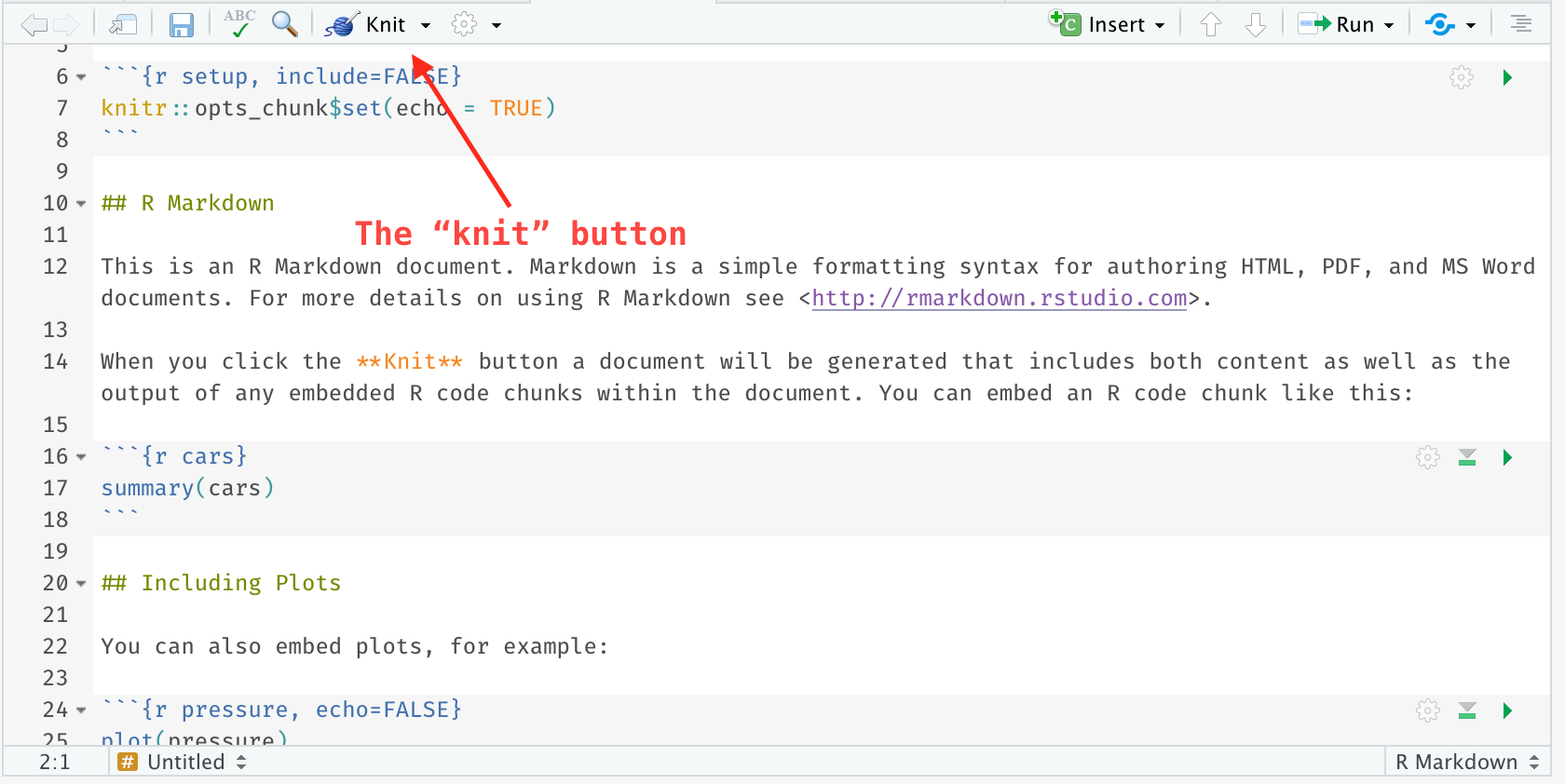
```These can be added automatically by clicking the “Insert” button (see top-right of the image below).
A chunk will be evaluated just like normal R code so everything we’ve learned in previous chapters applies. If there is output printed in the chunk (e.g., model output, a table, a ggplot2 figure), this will show up in the document.
But, say you, all I see is the code and text I’ve written. Where is this magical document that is formatted and has output all beautifully intertwined? Great question. This is something that most of us are not used to. For those that have used other word processors (like Microsoft Word, Apple’s Pages) you are using what is known as “WYSIWYG” (What You See Is What You Get). That is, you see how the document is going to look printed out while you type. This can have some advantages but it also can be very limiting.
R Markdown, on the other hand, must be “knit” to see what the formatted and evaluated document will look like. In RStudio, this is simple. There is a button at the top left of the scripting panel whenever an .Rmd (R Markdown) document is being displayed. By selecting this, our document will be created.
As we write, we can “knit” whenever we want to see what the document is looking like. Regardless of the type of document we choose, RStudio will find a way to show us the document. For example, if we choose html_document, a browser either within RStudio or a pop-up window will show the document.
With just this information, you can start writing reproducible documents. Congrats! Below I highlight a few additional features (among many, many others).
In-Line R Code
Beneficially, we can include in-line R code. Say we ran a model and we want to report the coefficient and p-value in the text. We can do this manually by just typing it in. But this comes with some problems if we update our data or analyses, as these values can change. If we aren’t careful, we can miss that and mis-report the updated values. Luckily, inline R code is pretty straightforward.
Let’s start with a quick model that we want to write about. We’ll use a form of a model we ran in Chapter 4, using minority status and marital status as a predictor of family size.
df$minority <- factor(ifelse(df$race == "White", 0, 1),
                      labels = c("White", "Minority"))
fit_reg <- lm(famsize ~ minority + marriage, df)
summary(fit_reg)
##
## Call:
## lm(formula = famsize ~ minority + marriage, data = df)
##
## Residuals:
## Min 1Q Median 3Q Max
## -2.34 -1.10 -0.34 0.88 4.36
##
## Coefficients:
## Estimate Std. Error t value Pr(>|t|)
## (Intercept) 2.8792 0.0381 75.48 < 2e-16 ***
## minorityMinority 0.4604 0.0421 10.93 < 2e-16 ***
## marriage2 -1.2353 0.0763 -16.19 < 2e-16 ***
## marriage3 -1.2195 0.0686 -17.79 < 2e-16 ***
## marriage4 -0.6341 0.1134 -5.59 2.4e-08 ***
## marriage5 -0.8840 0.0527 -16.76 < 2e-16 ***
## marriage6 -0.5277 0.0792 -6.66 3.0e-11 ***
## ---
## Signif. codes: 0 '***' 0.001 '**' 0.01 '*' 0.05 '.' 0.1 ' ' 1
##
## Residual standard error: 1.36 on 4447 degrees of freedom
## (178 observations deleted due to missingness)
## Multiple R-squared: 0.139, Adjusted R-squared: 0.138
## F-statistic: 120 on 6 and 4447 DF, p-value: <2e-16To make it easier to work with, we are going to use the broom package, which helps clean up the information that we’ll want to report.
tidy_fit <- broom::tidy(fit_reg)Let’s say we want to report the coefficient and the p-value on the minority variable. We can grab the coefficient by using: `r tidy_fit$estimate[2]`. This will evaluate the expression tidy_fit$estimate[2] when we knit and it will print out the value. One problem that can happen is that this coefficient is seven decimal places; probably a bit too far to report in the text. So let’s clean it up by doing: `r tidy_fit$estimate[2] %>% round(3)`, which rounds it to three decimal places. We may also want to format the p-value as well but let’s say if it is below .001, let’s report “p < .001”. We can do this by first running the code in a code chunk:
formatted_p <- ifelse(tidy_fit$p.value < .001, ## Condition
                      "< .001",  ## if condition is true
                      paste("=", tidy_fit$p.value[2] %>% round(3))) ## if condition is false
and then referring to it inline as so: `r formatted_p[2]`.
Below, is an example of how we could report this.
Controlling for marital status, minority status was associated with a family size
`r tidy_fit$estimate[2] %>% round(3)`individuals larger than non-minority families (p`r formatted_p[2]`).
which prints as:
Controlling for marital status, minority status was associated with a family size 0.46 individuals larger than non-minority families (p < .001).
Then, if we decide we want to change the covariates, or filter out extreme cases, these will automatically update to the most recent model.
Pre-formatted Documents
One of the main ideas is to be able to write without worrying about formatting. This is accomplished by using built-in formats provided by a number of great packages.
TABLE of PACKAGES HERE
Other Tricks
HTML code, figures, other knitr stuff
Important, Important
The document’s code must be fully self-contained. That means, anything you want it to run has to be in the document, regardless of what you’ve already run outside of knitting. For example, if we are testing our code and running it throughout, when we go to knit. It will re-run everything in the document and forget everything else you’ve done that is not in the document.
Some consequences of this:
- If you don’t include the code to read in the data set that you use in the document, the document won’t knit. Why? Because it doesn’t know where to get the data since you haven’t told the document where the data set is at.
- Errors anywhere in the code within the document will make it so it cannot knit. So if you have some experimental code that isn’t working yet, this could cause problems. Luckily, in the code chunk you can tell the document to ignore the code using
eval = FALSE:
```{r, eval = FALSE}
## R Code goes here
```
These are actually good things for you. This forces you to be fully reproducible in your work. R Markdown won’t let you skip steps in the data analysis. Although working through bugs can sometimes be annoying, this will ultimately bless your research. For if you can’t even reproduce your own research, then how can we expect any other researcher to reproduce it?
But this feature goes beyond that. In fact, it makes it so another research could reproduce your work by just downloading and running your R Markdown document. This removes all guesswork for others regarding your data analysis and reporting.
Going one step further would be to post your R Markdown document in a publically accessible repository, with (if possible) the data used in the R Markdown document. Although maybe intimidating showing others your code, this is actually an important step in making your research as reproducible as possible.
Apply It
This link contains a folder complete with an Rstudio project file, an RMarkdown file, and a few data files. Download it and unzip it to do the following steps.
Step 1
Open the Chapter9.Rproj file. This will open up RStudio for you.
Step 2
Once RStudio has started, in the panel on the lower-right, there is a Files tab. Click on that to see the project folder. You should see the data files and the Chapter9.Rmd file. Click on the Chapter9.Rmd file to open it. In this file, import the data and run each type of statistical analysis presented in this chapter.
Once that code is in the file, click the knit button. This will create an HTML file with the code and output knitted together into one nice document. This can be read into any browser and can be used to show your work in a clean document.
References
Begley, C. Glenn, and John P A Ioannidis. 2015. “Reproducibility in science: Improving the standard for basic and preclinical research.” Circulation Research 116 (1): 116–26. https://doi.org/10.1161/CIRCRESAHA.114.303819.
Cumming. 2014. “The new statistics: Why and how.” Psychological Science 25 (1): 7–29. https://doi.org/10.1177/0956797613504966.
Goodman, Steven N, Daniele Fanelli, and John P A Ioannidis. 2016. “What does research reproducibility mean?” Science Translational Medicine 8 (341): 1–6. https://doi.org/10.1126/scitranslmed.aaf5027.
Ioannidis, John P A. 2005. “Why most published research findings are false.” PLoS Medicine 2 (8): 0696–701. https://doi.org/10.1371/journal.pmed.0020124.
Munafò, Marcus R, Brian A Nosek, Dorothy V M Bishop, Katherine S Button, Christopher D Chambers, Nathalie Percie du Sert, Uri Simonsohn, et al. 2017. “A manifesto for reproducible science.” Nature Human Behaviour 1 (January): 1–9. https://doi.org/10.1038/s41562-016-0021.
Taylor, Jonathan, and Robert J Tibshirani. 2015. “Statistical learning and selective inference.” Proceedings of the National Academy of Sciences of the United States of America 112 (25). https://doi.org/10.1073/pnas.1507583112.